


Line plots with pgfplots
Add one \addplot per line inside an axis; style each with options such as red, dashed, thick or mark=square*, or let the cycle list choose a style for you.
Several lines in one axis
Each \addplot adds a series. Without options, the series take their style from the cycle list in turn. With \addplot+[...] you keep that style and change one part of it.
Three series from the default cycle list
\begin{tikzpicture}
  \begin{axis}[xlabel=Week, ylabel=Orders, legend pos=north west]
    \addplot coordinates {(1,12) (2,18) (3,25) (4,31) (5,44)};
    \addplot coordinates {(1,10) (2,14) (3,15) (4,21) (5,24)};
    \addplot+[dashed] coordinates {(1,5) (2,9) (3,8) (4,12) (5,13)};
    \legend{Erika, Hans, John}
  \end{axis}
\end{tikzpicture}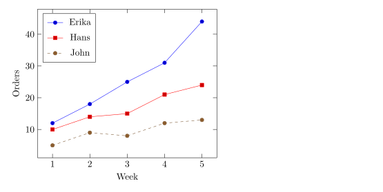
Line styles and marks
Options after \addplot set the colour, the line and the marks. You can combine them freely.
| Option | Values | In Scissor LaTeX |
|---|---|---|
| colour | red, blue!60!black, color=teal, any xcolor name or mix | Works |
| line width | ultra thin, very thin, thin, semithick, thick, very thick, ultra thick, line width=1.5pt | Works |
| dash pattern | solid, dashed, dotted, densely dashed, loosely dotted, dashdotted, dash pattern=on 4pt off 2pt | Works |
mark= | *, o, square*, square, triangle*, triangle, diamond*, diamond, x, +, star, pentagon*, asterisk, otimes*, |, -, none | Works |
mark size=3pt | radius of the mark | Works |
mark options={fill=white} | style of the marks only | Works |
mark repeat=2 | a mark on every second point | Works |
no marks, only marks | lines only, marks only | Works |
Colours, dash patterns and marks
\begin{tikzpicture}
  \begin{axis}[domain=0:4, samples=9, legend pos=outer north east]
    \addplot[blue, thick, mark=*] {x};
    \addplot[red, dashed, mark=square*, mark options={fill=white}] {x^1.5/2};
    \addplot[teal, densely dotted, very thick] {sqrt(x)};
    \addplot[orange, mark=triangle*, mark size=3pt, only marks] {4 - x};
    \legend{linear, power, root, falling}
  \end{axis}
\end{tikzpicture}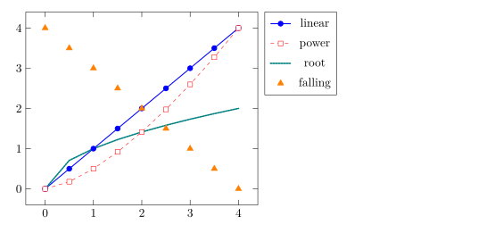
Marks are always drawn with solid lines, even on a dashed series, as in pgfplots.
Choosing a cycle list
A cycle list is the sequence of styles that plain \addplot commands use. Pick a built-in one with cycle list name, or write your own with cycle list.
The black white cycle list, and a custom one
\begin{tikzpicture}
  \begin{axis}[cycle list name=black white, width=6.5cm, height=5cm, title={black white}]
    \addplot coordinates {(0,0) (1,1) (2,4)};
    \addplot coordinates {(0,1) (1,2) (2,2)};
    \addplot coordinates {(0,2) (1,0) (2,1)};
  \end{axis}
\end{tikzpicture}
\begin{tikzpicture}
  \begin{axis}[cycle list={{red, thick}, {blue, dashed}}, width=6.5cm, height=5cm, title={custom}]
    \addplot coordinates {(0,0) (1,1) (2,4)};
    \addplot coordinates {(0,1) (1,2) (2,2)};
  \end{axis}
\end{tikzpicture}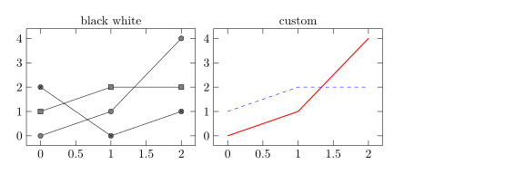
Built-in names that work: color (the default), exotic, black white, mark list and linestyles. \pgfplotscreateplotcyclelist{name}{...} in the preamble defines a list you can reuse.
Smooth curves and steps
smooth draws a curve through the points instead of straight segments; tension (default 0.55) controls how round it is. const plot draws a step function that holds each value until the next point.
smooth and const plot
\begin{tikzpicture}
  \begin{axis}[ymin=0, legend pos=north west]
    \addplot+[smooth] coordinates {(0,1) (1,2.5) (2,1.8) (3,3.2) (4,2.4)};
    \addplot+[const plot] coordinates {(0,0.5) (1,1) (2,1.5) (3,1.2) (4,2)};
    \legend{smooth, const plot}
  \end{axis}
\end{tikzpicture}
Functions in degrees and radians
Formulas use pgfmath: + - * / ^, parentheses, sqrt, exp, ln, abs, min, max, sin, cos, tan and more, with pi and e as constants. Angles are in degrees, so convert radians with deg(x).
sin and cos over one period
\begin{tikzpicture}
  \begin{axis}[domain=0:2*pi, samples=80, xlabel=$t$,
               xtick={0,1.5708,3.1416,4.7124,6.2832},
               xticklabels={$0$,$\frac{\pi}{2}$,$\pi$,$\frac{3\pi}{2}$,$2\pi$},
               legend pos=south west]
    \addplot[blue, thick] {sin(deg(x))};
    \addplot[red, thick, dashed] {cos(deg(x))};
    \legend{$\sin t$, $\cos t$}
  \end{axis}
\end{tikzpicture}
Parametric curves
To plot a curve given by x(t) and y(t), write both formulas in parentheses, separated by a comma, and set variable=t.
A Lissajous curve
\begin{tikzpicture}
  \begin{axis}[axis lines=middle, xmin=-1.3, xmax=1.3, ymin=-1.3, ymax=1.3]
    \addplot[purple, thick, domain=0:360, samples=120, variable=t]
      ({cos(t)}, {sin(2*t)});
  \end{axis}
\end{tikzpicture}
Gaps in a curve
A function such as 1/x shoots off to infinity. restrict y to domain drops the points outside a range, and unbounded coords=jump breaks the line there instead of joining the two branches. Put both on the \addplot.
1/x with a break at zero
\begin{tikzpicture}
  \begin{axis}[ymin=-10, ymax=10, axis lines=middle]
    \addplot[blue, thick, domain=-3:3, samples=200,
             restrict y to domain=-10:10, unbounded coords=jump] {1/x};
  \end{axis}
\end{tikzpicture}
What differs from a TeX installation
The pgfplots manual on CTAN describes every option: ctan.org/pkg/pgfplots. For points without lines, see scatter plots.
See also pgfplots basics, Logarithmic axes, Group plots and Data from CSV.
Questions and answers
How do I plot a function in LaTeX?
Write \addplot[domain=a:b, samples=n] {formula}; inside an axis, using x as the variable, for example {x^2 - 1}.
How do I remove the marks from a line?
Add no marks to the \addplot options, or give options without + (for example \addplot[blue]), which draws a plain line.
Why does sin(x) look almost flat?
pgfplots reads the angle in degrees, so sin(x) on 0 to 6 covers only 6 degrees. Write sin(deg(x)).
Every example on this page is typeset by Scissor LaTeX when the site is built. Last updated 2026-11-06.