


גרפי קווים עם pgfplots
מוסיפים \addplot אחד לכל קו בתוך axis; מעצבים כל אחד באפשרויות כמו red, dashed, thick או mark=square*, או נותנים לרשימת המחזור לבחור סגנון בשבילך.
כמה קווים על ציר אחד
כל \addplot מוסיף סדרה. בלי אפשרויות, הסדרות מקבלות את הסגנון שלהן מרשימת המחזור (cycle list) לפי הסדר. עם \addplot+[...] שומרים על הסגנון הזה ומשנים רק חלק ממנו.
שלוש סדרות מרשימת המחזור שמוגדרת כברירת מחדל
\begin{tikzpicture}
  \begin{axis}[xlabel=Week, ylabel=Orders, legend pos=north west]
    \addplot coordinates {(1,12) (2,18) (3,25) (4,31) (5,44)};
    \addplot coordinates {(1,10) (2,14) (3,15) (4,21) (5,24)};
    \addplot+[dashed] coordinates {(1,5) (2,9) (3,8) (4,12) (5,13)};
    \legend{Erika, Hans, John}
  \end{axis}
\end{tikzpicture}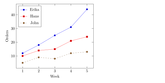
סגנונות קו וסמנים
אפשרויות אחרי \addplot קובעות את הצבע, את הקו ואת הסמנים. אפשר לשלב ביניהן בחופשיות.
| אפשרות | ערכים | ב-Scissor LaTeX |
|---|---|---|
| צבע | red, blue!60!black, color=teal, כל שם צבע או תערובת של xcolor | עובד |
| עובי קו | ultra thin, very thin, thin, semithick, thick, very thick, ultra thick, line width=1.5pt | עובד |
| דוגמת קו | solid, dashed, dotted, densely dashed, loosely dotted, dashdotted, dash pattern=on 4pt off 2pt | עובד |
mark= | *, o, square*, square, triangle*, triangle, diamond*, diamond, x, +, star, pentagon*, asterisk, otimes*, |, -, none | עובד |
mark size=3pt | הרדיוס של הסמן | עובד |
mark options={fill=white} | סגנון של הסמנים בלבד | עובד |
mark repeat=2 | סמן על כל נקודה שנייה | עובד |
no marks, only marks | קווים בלבד, סמנים בלבד | עובד |
צבעים, דוגמאות קו וסמנים
\begin{tikzpicture}
  \begin{axis}[domain=0:4, samples=9, legend pos=outer north east]
    \addplot[blue, thick, mark=*] {x};
    \addplot[red, dashed, mark=square*, mark options={fill=white}] {x^1.5/2};
    \addplot[teal, densely dotted, very thick] {sqrt(x)};
    \addplot[orange, mark=triangle*, mark size=3pt, only marks] {4 - x};
    \legend{linear, power, root, falling}
  \end{axis}
\end{tikzpicture}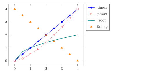
סמנים תמיד מצוירים בקווים רציפים, גם על סדרה מקווקוות, כמו ב-pgfplots.
בחירת רשימת מחזור
רשימת מחזור היא רצף הסגנונות שפקודות \addplot פשוטות משתמשות בהם. בוחרים רשימה מובנית עם cycle list name, או כותבים רשימה משלך עם cycle list.
רשימת המחזור black white, ורשימה מותאמת אישית
\begin{tikzpicture}
  \begin{axis}[cycle list name=black white, width=6.5cm, height=5cm, title={black white}]
    \addplot coordinates {(0,0) (1,1) (2,4)};
    \addplot coordinates {(0,1) (1,2) (2,2)};
    \addplot coordinates {(0,2) (1,0) (2,1)};
  \end{axis}
\end{tikzpicture}
\begin{tikzpicture}
  \begin{axis}[cycle list={{red, thick}, {blue, dashed}}, width=6.5cm, height=5cm, title={custom}]
    \addplot coordinates {(0,0) (1,1) (2,4)};
    \addplot coordinates {(0,1) (1,2) (2,2)};
  \end{axis}
\end{tikzpicture}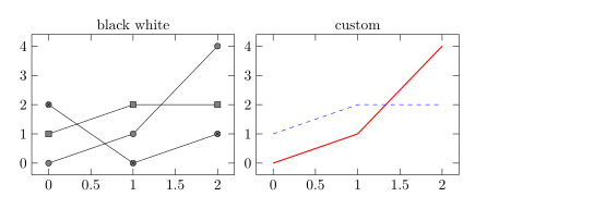
השמות המובנים שעובדים: color (ברירת המחדל), exotic, black white, mark list ו-linestyles. \pgfplotscreateplotcyclelist{name}{...} בפתיח מגדיר רשימה שאפשר להשתמש בה שוב.
עקומות חלקות ומדרגות
smooth מצייר עקומה דרך הנקודות במקום קטעים ישרים; tension (ברירת מחדל 0.55) קובע עד כמה היא מעוגלת. const plot מצייר פונקציית מדרגות שמחזיקה כל ערך עד הנקודה הבאה.
smooth ו-const plot
\begin{tikzpicture}
  \begin{axis}[ymin=0, legend pos=north west]
    \addplot+[smooth] coordinates {(0,1) (1,2.5) (2,1.8) (3,3.2) (4,2.4)};
    \addplot+[const plot] coordinates {(0,0.5) (1,1) (2,1.5) (3,1.2) (4,2)};
    \legend{smooth, const plot}
  \end{axis}
\end{tikzpicture}
פונקציות במעלות וברדיאנים
נוסחאות משתמשות ב-pgfmath: + - * / ^, סוגריים, sqrt, exp, ln, abs, min, max, sin, cos, tan ועוד, עם pi ו-e כקבועים. זוויות הן במעלות, ולכן ממירים רדיאנים עם deg(x).
sin ו-cos לאורך מחזור אחד
\begin{tikzpicture}
  \begin{axis}[domain=0:2*pi, samples=80, xlabel=$t$,
               xtick={0,1.5708,3.1416,4.7124,6.2832},
               xticklabels={$0$,$\frac{\pi}{2}$,$\pi$,$\frac{3\pi}{2}$,$2\pi$},
               legend pos=south west]
    \addplot[blue, thick] {sin(deg(x))};
    \addplot[red, thick, dashed] {cos(deg(x))};
    \legend{$\sin t$, $\cos t$}
  \end{axis}
\end{tikzpicture}
עקומות פרמטריות
כדי לצייר עקומה שנתונה על ידי x(t) ו-y(t), כותבים את שתי הנוסחאות בסוגריים, מופרדות בפסיק, וקובעים variable=t.
עקומת ליסז'ו
\begin{tikzpicture}
  \begin{axis}[axis lines=middle, xmin=-1.3, xmax=1.3, ymin=-1.3, ymax=1.3]
    \addplot[purple, thick, domain=0:360, samples=120, variable=t]
      ({cos(t)}, {sin(2*t)});
  \end{axis}
\end{tikzpicture}
רווחים בעקומה
פונקציה כמו 1/x בורחת לאינסוף. restrict y to domain משמיט את הנקודות שמחוץ לטווח, ו-unbounded coords=jump שובר שם את הקו במקום לחבר את שני הענפים. שמים את שתיהן על ה-\addplot.
1/x עם שבירה באפס
\begin{tikzpicture}
  \begin{axis}[ymin=-10, ymax=10, axis lines=middle]
    \addplot[blue, thick, domain=-3:3, samples=200,
             restrict y to domain=-10:10, unbounded coords=jump] {1/x};
  \end{axis}
\end{tikzpicture}
מה שונה מהתקנת TeX
מדריך pgfplots ב-CTAN מתאר כל אפשרות: ctan.org/pkg/pgfplots. לנקודות בלי קווים, ראו גרפי פיזור.
ראו גם יסודות pgfplots, צירים לוגריתמיים, קבוצות גרפים ונתונים מקובץ CSV.
שאלות ותשובות
איך מציירים פונקציה ב-LaTeX?
כותבים \addplot[domain=a:b, samples=n] {formula}; בתוך axis, עם x בתור המשתנה, למשל {x^2 - 1}.
איך מסירים את הסמנים מקו?
מוסיפים no marks לאפשרויות של \addplot, או נותנים אפשרויות בלי + (למשל \addplot[blue]), וזה מצייר קו פשוט.
למה sin(x) נראה כמעט שטוח?
pgfplots קורא את הזווית במעלות, ולכן sin(x) בין 0 ל-6 מכסה רק 6 מעלות. כותבים sin(deg(x)).
כל דוגמה בדף הזה מסודרת על ידי Scissor LaTeX בזמן בניית האתר. עודכן לאחרונה: 2026-11-07.