


Error bars with pgfplots
Add error bars/.cd, y dir=both, y explicit to the \addplot options and write each error after its point as +- (0, error), or read the errors from a table column with y error=.
Errors written with the points
Error bars are switched on per \addplot. The keys after error bars/.cd say in which direction to draw them and where the values come from. With y explicit, each point carries its own error after +-.
Symmetric y errors from the coordinates
\begin{tikzpicture}
  \begin{axis}[xlabel={Length (m)}, ylabel={Period (s)}]
    \addplot+[error bars/.cd, y dir=both, y explicit]
      coordinates {
        (0.2,0.90) +- (0,0.05)
        (0.4,1.27) +- (0,0.04)
        (0.6,1.55) +- (0,0.06)
        (0.8,1.80) +- (0,0.05)
        (1.0,2.01) +- (0,0.07)
      };
  \end{axis}
\end{tikzpicture}
In +- (ex, ey) the first number is the x error and the second the y error. Only the directions you switch on are drawn.
Errors from a table column
When the data is a table, name the error column with y error=. The same works with a file, for example table[x=t, y=v, y error=dv, col sep=comma] {data.csv}.
y errors read from a column
\begin{tikzpicture}
  \begin{axis}[xlabel={Dose}, ylabel={Response}, ymin=0]
    \addplot+[only marks, error bars/.cd, y dir=both, y explicit]
      table[x=dose, y=mean, y error=sd] {
        dose mean sd
        1    2.1  0.3
        2    3.4  0.4
        4    5.0  0.6
        8    6.2  0.5
      };
  \end{axis}
\end{tikzpicture}
One-sided and fixed errors
y dir=plus or y dir=minus draws only the upper or the lower half. Instead of explicit values, y fixed=0.2 gives every point the same error, and y fixed relative=0.1 an error of 10% of its value.
Upper errors only, and a relative error
\begin{tikzpicture}
  \begin{axis}[ymin=0, legend pos=north west]
    \addplot+[error bars/.cd, y dir=plus, y fixed=0.4]
      coordinates {(1,2) (2,3) (3,3.5) (4,4.4)};
    \addplot+[error bars/.cd, y dir=both, y fixed relative=0.1]
      coordinates {(1,1) (2,1.6) (3,2.2) (4,2.5)};
    \legend{fixed $\pm 0.4$ (upper), relative 10\%}
  \end{axis}
\end{tikzpicture}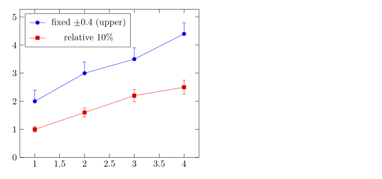
Different errors above and below
Write += (0, up) for the upper error and -= (0, down) for the lower one.
Asymmetric errors
\begin{tikzpicture}
  \begin{axis}[width=7cm, height=5cm, xmin=0.5, xmax=3.5]
    \addplot+[only marks, error bars/.cd, y dir=both, y explicit]
      coordinates {
        (1,2.0) += (0,0.5) -= (0,0.1)
        (2,3.0) += (0,0.2) -= (0,0.6)
        (3,2.6) += (0,0.3) -= (0,0.3)
      };
  \end{axis}
\end{tikzpicture}
Errors in x and y
Switch on both directions with x dir and y dir. error bar style styles the bars.
Error bars in both directions
\begin{tikzpicture}
  \begin{axis}[xlabel=$x$, ylabel=$y$]
    \addplot+[only marks, mark=square*,
              error bars/.cd,
                x dir=both, x explicit,
                y dir=both, y explicit,
                error bar style={red, thick}]
      coordinates {
        (1.0,1.2) +- (0.15,0.20)
        (2.0,2.1) +- (0.20,0.15)
        (3.0,2.8) +- (0.10,0.30)
      };
  \end{axis}
\end{tikzpicture}
Error bands with fill between
For a continuous uncertainty, shade the area between an upper and a lower curve. Load the fillbetween library, name both curves with name path, and fill between them.
A shaded band around a curve
\documentclass{article}
\usepackage{pgfplots}
\usepgfplotslibrary{fillbetween}
\begin{document}
\begin{tikzpicture}
  \begin{axis}[domain=0:4, samples=40, xlabel=$t$, ylabel=$y$]
    \addplot[name path=upper, draw=none] {exp(-0.5*x) + 0.1 + 0.05*x};
    \addplot[name path=lower, draw=none] {exp(-0.5*x) - 0.1 - 0.05*x};
    \addplot[blue!20] fill between[of=upper and lower];
    \addplot[blue, thick] {exp(-0.5*x)};
  \end{axis}
\end{tikzpicture}
\end{document}
Error bar options
| Option | What it does | In Scissor LaTeX |
|---|---|---|
y dir=both, plus, minus, none | which half of the bar to draw (also x dir) | Works |
y explicit, x explicit | errors from +- in coordinates or from a table column | Works |
y error=col, x error=col, y error index=n | the table column with the errors | Works |
+= (ex,ey), -= (ex,ey) | separate upper and lower errors in coordinates | Works |
y fixed=v, y fixed relative=r | the same error for every point | Works |
error bar style={..} | colour and line width of the bars | Works |
error mark=.., error mark options={..} | the cap at each end | Accepted, but the cap is always a short line |
What differs from a TeX installation
The pgfplots manual describes error bars in its section on error bars: ctan.org/pkg/pgfplots.
See also Bar charts, Scatter plots and Data from CSV.
Questions and answers
How do I add error bars in pgfplots?
Write \addplot+[error bars/.cd, y dir=both, y explicit] coordinates {(1,2) +- (0,0.3) ...};. The second number after +- is the y error.
How do I read error bars from a CSV file?
Add y error=column to the table options, together with y explicit in the error bar options: table[x=a, y=b, y error=c, col sep=comma] {file.csv}.
Can error bars be different above and below?
Yes. Write += (0, up) and -= (0, down) after the point instead of +-, as in (1,2) += (0,0.5) -= (0,0.1).
Every example on this page is typeset by Scissor LaTeX when the site is built. Last updated 2026-11-06.