


用 pgfplots 绘制折线图
在 axis 中为每条线添加一个 \addplot;用 red、dashed、thick 或 mark=square* 等选项设置各自的样式,或者让循环列表为你选择样式。
一个坐标轴中的多条线
每个 \addplot 添加一个系列。不带选项时,各系列依次从循环列表中获取样式。使用 \addplot+[...] 可以保留该样式,只更改其中一部分。
来自默认循环列表的三个系列
\begin{tikzpicture}
  \begin{axis}[xlabel=Week, ylabel=Orders, legend pos=north west]
    \addplot coordinates {(1,12) (2,18) (3,25) (4,31) (5,44)};
    \addplot coordinates {(1,10) (2,14) (3,15) (4,21) (5,24)};
    \addplot+[dashed] coordinates {(1,5) (2,9) (3,8) (4,12) (5,13)};
    \legend{Erika, Hans, John}
  \end{axis}
\end{tikzpicture}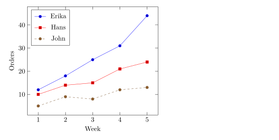
线型和标记
\addplot 之后的选项设置颜色、线条和标记。它们可以自由组合。
| 选项 | 取值 | 在 Scissor LaTeX 中 |
|---|---|---|
| 颜色 | red、blue!60!black、color=teal,任意 xcolor 颜色名或混合色 | 支持 |
| 线宽 | ultra thin、very thin、thin、semithick、thick、very thick、ultra thick、line width=1.5pt | 支持 |
| 虚线样式 | solid、dashed、dotted、densely dashed、loosely dotted、dashdotted、dash pattern=on 4pt off 2pt | 支持 |
mark= | *、o、square*、square、triangle*、triangle、diamond*、diamond、x、+、star、pentagon*、asterisk、otimes*、|、-、none | 支持 |
mark size=3pt | 标记的半径 | 支持 |
mark options={fill=white} | 仅设置标记的样式 | 支持 |
mark repeat=2 | 每隔一个点画一个标记 | 支持 |
no marks、only marks | 只画线、只画标记 | 支持 |
颜色、虚线样式和标记
\begin{tikzpicture}
  \begin{axis}[domain=0:4, samples=9, legend pos=outer north east]
    \addplot[blue, thick, mark=*] {x};
    \addplot[red, dashed, mark=square*, mark options={fill=white}] {x^1.5/2};
    \addplot[teal, densely dotted, very thick] {sqrt(x)};
    \addplot[orange, mark=triangle*, mark size=3pt, only marks] {4 - x};
    \legend{linear, power, root, falling}
  \end{axis}
\end{tikzpicture}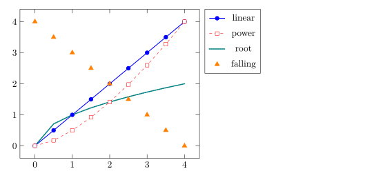
和 pgfplots 中一样,即使系列是虚线,标记也总是用实线绘制。
选择循环列表
循环列表是不带选项的 \addplot 命令依次使用的样式序列。用 cycle list name 选择一个内置列表,或用 cycle list 自己编写。
black white 循环列表和一个自定义列表
\begin{tikzpicture}
  \begin{axis}[cycle list name=black white, width=6.5cm, height=5cm, title={black white}]
    \addplot coordinates {(0,0) (1,1) (2,4)};
    \addplot coordinates {(0,1) (1,2) (2,2)};
    \addplot coordinates {(0,2) (1,0) (2,1)};
  \end{axis}
\end{tikzpicture}
\begin{tikzpicture}
  \begin{axis}[cycle list={{red, thick}, {blue, dashed}}, width=6.5cm, height=5cm, title={custom}]
    \addplot coordinates {(0,0) (1,1) (2,4)};
    \addplot coordinates {(0,1) (1,2) (2,2)};
  \end{axis}
\end{tikzpicture}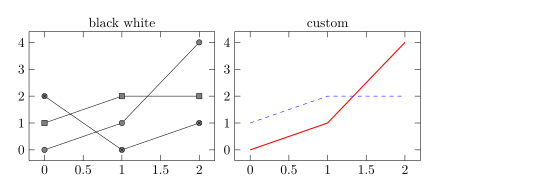
可用的内置名称有:color(默认)、exotic、black white、mark list 和 linestyles。在导言区用 \pgfplotscreateplotcyclelist{name}{...} 可以定义一个可重复使用的列表。
平滑曲线和阶梯
smooth 用一条曲线穿过各点,而不是用直线段连接;tension(默认 0.55)控制曲线的圆滑程度。const plot 绘制阶梯函数,每个值保持到下一个点为止。
smooth 和 const plot
\begin{tikzpicture}
  \begin{axis}[ymin=0, legend pos=north west]
    \addplot+[smooth] coordinates {(0,1) (1,2.5) (2,1.8) (3,3.2) (4,2.4)};
    \addplot+[const plot] coordinates {(0,0.5) (1,1) (2,1.5) (3,1.2) (4,2)};
    \legend{smooth, const plot}
  \end{axis}
\end{tikzpicture}
角度制和弧度制的函数
公式使用 pgfmath:+ - * / ^、括号、sqrt、exp、ln、abs、min、max、sin、cos、tan 等,常数有 pi 和 e。角度使用角度制,所以弧度要用 deg(x) 转换。
一个周期内的 sin 和 cos
\begin{tikzpicture}
  \begin{axis}[domain=0:2*pi, samples=80, xlabel=$t$,
               xtick={0,1.5708,3.1416,4.7124,6.2832},
               xticklabels={$0$,$\frac{\pi}{2}$,$\pi$,$\frac{3\pi}{2}$,$2\pi$},
               legend pos=south west]
    \addplot[blue, thick] {sin(deg(x))};
    \addplot[red, thick, dashed] {cos(deg(x))};
    \legend{$\sin t$, $\cos t$}
  \end{axis}
\end{tikzpicture}
参数曲线
要绘制由 x(t) 和 y(t) 给出的曲线,把两个公式写在圆括号中,用逗号分隔,并设置 variable=t。
李萨如曲线
\begin{tikzpicture}
  \begin{axis}[axis lines=middle, xmin=-1.3, xmax=1.3, ymin=-1.3, ymax=1.3]
    \addplot[purple, thick, domain=0:360, samples=120, variable=t]
      ({cos(t)}, {sin(2*t)});
  \end{axis}
\end{tikzpicture}
曲线中的间断
像 1/x 这样的函数会趋于无穷。restrict y to domain 会去掉范围之外的点,unbounded coords=jump 会在那里断开线条,而不是把两个分支连起来。两者都写在 \addplot 上。
在零处断开的 1/x
\begin{tikzpicture}
  \begin{axis}[ymin=-10, ymax=10, axis lines=middle]
    \addplot[blue, thick, domain=-3:3, samples=200,
             restrict y to domain=-10:10, unbounded coords=jump] {1/x};
  \end{axis}
\end{tikzpicture}
与 TeX 发行版的不同之处
CTAN 上的 pgfplots 手册介绍了所有选项:ctan.org/pkg/pgfplots。只画点不画线,请参阅散点图。
另请参阅 pgfplots 基础、对数坐标轴、组图和来自 CSV 的数据。
常见问题
如何在 LaTeX 中绘制函数?
在 axis 中写 \addplot[domain=a:b, samples=n] {formula};,以 x 为变量,例如 {x^2 - 1}。
如何去掉线上的标记?
在 \addplot 的选项中加 no marks,或者不带 + 给出选项(例如 \addplot[blue]),这样会画出一条普通的线。
为什么 sin(x) 看起来几乎是平的?
pgfplots 按角度制读取角度,所以 0 到 6 上的 sin(x) 只覆盖 6 度。请写 sin(deg(x))。
本页的每个示例都在构建网站时由 Scissor LaTeX 排版。 最后更新:2026-11-07