


pgfplots کے ساتھ لائن پلاٹس
axis کے اندر ہر لکیر کے لیے ایک \addplot شامل کریں؛ ہر ایک کو red، dashed، thick یا mark=square* جیسے آپشنز سے سنواریں، یا سائیکل لسٹ کو آپ کے لیے انداز چننے دیں۔
ایک محور میں کئی لکیریں
ہر \addplot ایک سیریز شامل کرتا ہے۔ آپشنز کے بغیر سیریز باری باری سائیکل لسٹ سے اپنا انداز لیتی ہیں۔ \addplot+[...] سے آپ وہ انداز برقرار رکھتے ہیں اور اس کا ایک حصہ بدلتے ہیں۔
طے شدہ سائیکل لسٹ سے تین سیریز
\begin{tikzpicture}
  \begin{axis}[xlabel=Week, ylabel=Orders, legend pos=north west]
    \addplot coordinates {(1,12) (2,18) (3,25) (4,31) (5,44)};
    \addplot coordinates {(1,10) (2,14) (3,15) (4,21) (5,24)};
    \addplot+[dashed] coordinates {(1,5) (2,9) (3,8) (4,12) (5,13)};
    \legend{Erika, Hans, John}
  \end{axis}
\end{tikzpicture}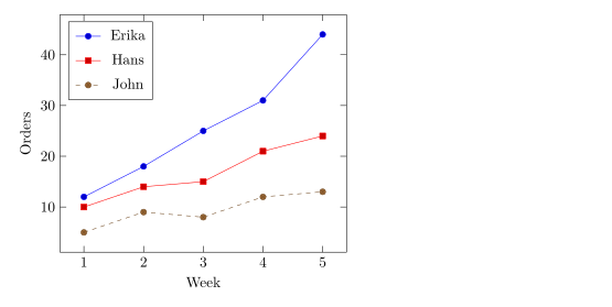
لکیر کے انداز اور نشانات
\addplot کے بعد آپشنز رنگ، لکیر اور نشانات طے کرتے ہیں۔ آپ انہیں آزادی سے ملا سکتے ہیں۔
| آپشن | قدریں | Scissor LaTeX میں |
|---|---|---|
| رنگ | red، blue!60!black، color=teal، کوئی بھی xcolor نام یا آمیزہ | کام کرتا ہے |
| لکیر کی موٹائی | ultra thin، very thin، thin، semithick، thick، very thick، ultra thick، line width=1.5pt | کام کرتا ہے |
| ڈیش پیٹرن | solid، dashed، dotted، densely dashed، loosely dotted، dashdotted، dash pattern=on 4pt off 2pt | کام کرتا ہے |
mark= | *، o، square*، square، triangle*، triangle، diamond*، diamond، x، +، star، pentagon*، asterisk، otimes*، |، -، none | کام کرتا ہے |
mark size=3pt | نشان کا رداس | کام کرتا ہے |
mark options={fill=white} | صرف نشانات کا انداز | کام کرتا ہے |
mark repeat=2 | ہر دوسرے پوائنٹ پر ایک نشان | کام کرتا ہے |
no marks، only marks | صرف لکیریں، صرف نشانات | کام کرتا ہے |
رنگ، ڈیش پیٹرن اور نشانات
\begin{tikzpicture}
  \begin{axis}[domain=0:4, samples=9, legend pos=outer north east]
    \addplot[blue, thick, mark=*] {x};
    \addplot[red, dashed, mark=square*, mark options={fill=white}] {x^1.5/2};
    \addplot[teal, densely dotted, very thick] {sqrt(x)};
    \addplot[orange, mark=triangle*, mark size=3pt, only marks] {4 - x};
    \legend{linear, power, root, falling}
  \end{axis}
\end{tikzpicture}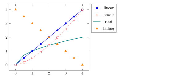
نشانات ہمیشہ ٹھوس لکیروں سے بنتے ہیں، ڈیشڈ سیریز پر بھی، بالکل pgfplots کی طرح۔
سائیکل لسٹ کا انتخاب
سائیکل لسٹ اندازوں کا وہ سلسلہ ہے جو سادہ \addplot کمانڈز استعمال کرتی ہیں۔ cycle list name سے کوئی بلٹ اِن لسٹ چنیں، یا cycle list سے اپنی لسٹ لکھیں۔
black white سائیکل لسٹ، اور ایک اپنی بنائی ہوئی
\begin{tikzpicture}
  \begin{axis}[cycle list name=black white, width=6.5cm, height=5cm, title={black white}]
    \addplot coordinates {(0,0) (1,1) (2,4)};
    \addplot coordinates {(0,1) (1,2) (2,2)};
    \addplot coordinates {(0,2) (1,0) (2,1)};
  \end{axis}
\end{tikzpicture}
\begin{tikzpicture}
  \begin{axis}[cycle list={{red, thick}, {blue, dashed}}, width=6.5cm, height=5cm, title={custom}]
    \addplot coordinates {(0,0) (1,1) (2,4)};
    \addplot coordinates {(0,1) (1,2) (2,2)};
  \end{axis}
\end{tikzpicture}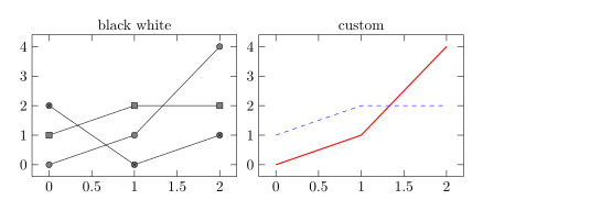
کام کرنے والے بلٹ اِن نام: color (طے شدہ)، exotic، black white، mark list اور linestyles۔ ابتدائیے میں \pgfplotscreateplotcyclelist{name}{...} ایسی لسٹ بناتا ہے جسے آپ بار بار استعمال کر سکتے ہیں۔
ہموار خم اور سیڑھیاں
smooth سیدھے ٹکڑوں کی بجائے پوائنٹس سے گزرتا خم بناتا ہے؛ tension (طے شدہ 0.55) طے کرتا ہے کہ خم کتنا گول ہو۔ const plot سیڑھی نما فنکشن بناتا ہے جو ہر قدر کو اگلے پوائنٹ تک برقرار رکھتا ہے۔
smooth اور const plot
\begin{tikzpicture}
  \begin{axis}[ymin=0, legend pos=north west]
    \addplot+[smooth] coordinates {(0,1) (1,2.5) (2,1.8) (3,3.2) (4,2.4)};
    \addplot+[const plot] coordinates {(0,0.5) (1,1) (2,1.5) (3,1.2) (4,2)};
    \legend{smooth, const plot}
  \end{axis}
\end{tikzpicture}
ڈگری اور ریڈین میں فنکشنز
فارمولے pgfmath استعمال کرتے ہیں: + - * / ^، قوسین، sqrt، exp، ln، abs، min، max، sin، cos، tan اور مزید، اور مستقل قدروں کے طور پر pi اور e۔ زاویے ڈگری میں ہوتے ہیں، اس لیے ریڈین کو deg(x) سے بدلیں۔
ایک دور پر sin اور cos
\begin{tikzpicture}
  \begin{axis}[domain=0:2*pi, samples=80, xlabel=$t$,
               xtick={0,1.5708,3.1416,4.7124,6.2832},
               xticklabels={$0$,$\frac{\pi}{2}$,$\pi$,$\frac{3\pi}{2}$,$2\pi$},
               legend pos=south west]
    \addplot[blue, thick] {sin(deg(x))};
    \addplot[red, thick, dashed] {cos(deg(x))};
    \legend{$\sin t$, $\cos t$}
  \end{axis}
\end{tikzpicture}
پیرامیٹرک خم
x(t) اور y(t) سے دیے گئے خم کو پلاٹ کرنے کے لیے دونوں فارمولے قوسین میں، کوما سے الگ کر کے لکھیں، اور variable=t مقرر کریں۔
ایک Lissajous خم
\begin{tikzpicture}
  \begin{axis}[axis lines=middle, xmin=-1.3, xmax=1.3, ymin=-1.3, ymax=1.3]
    \addplot[purple, thick, domain=0:360, samples=120, variable=t]
      ({cos(t)}, {sin(2*t)});
  \end{axis}
\end{tikzpicture}
خم میں خلا
1/x جیسا فنکشن لامتناہی کی طرف بھاگ جاتا ہے۔ restrict y to domain کسی حد سے باہر کے پوائنٹس ہٹا دیتا ہے، اور unbounded coords=jump دونوں شاخوں کو جوڑنے کی بجائے وہاں لکیر توڑ دیتا ہے۔ دونوں کو \addplot پر لگائیں۔
صفر پر وقفے کے ساتھ 1/x
\begin{tikzpicture}
  \begin{axis}[ymin=-10, ymax=10, axis lines=middle]
    \addplot[blue, thick, domain=-3:3, samples=200,
             restrict y to domain=-10:10, unbounded coords=jump] {1/x};
  \end{axis}
\end{tikzpicture}
TeX انسٹالیشن سے کیا مختلف ہے
CTAN پر pgfplots دستی ہر آپشن کی وضاحت کرتی ہے: ctan.org/pkg/pgfplots۔ لکیروں کے بغیر پوائنٹس کے لیے سکیٹر پلاٹس دیکھیں۔
یہ بھی دیکھیں: pgfplots کی بنیادی باتیں، لاگرتھمی محور، گروپ پلاٹس اور CSV سے ڈیٹا۔
سوالات اور جوابات
میں LaTeX میں فنکشن کیسے پلاٹ کروں؟
axis کے اندر \addplot[domain=a:b, samples=n] {formula}; لکھیں، متغیر کے طور پر x استعمال کرتے ہوئے، مثلاً {x^2 - 1}۔
میں لکیر سے نشانات کیسے ہٹاؤں؟
\addplot کے آپشنز میں no marks شامل کریں، یا + کے بغیر آپشنز دیں (مثلاً \addplot[blue])، جو سادہ لکیر بناتا ہے۔
sin(x) تقریباً سیدھا کیوں دکھتا ہے؟
pgfplots زاویہ ڈگری میں پڑھتا ہے، اس لیے 0 سے 6 تک sin(x) صرف 6 ڈگری کا احاطہ کرتا ہے۔ sin(deg(x)) لکھیں۔
اس صفحے کی ہر مثال سائٹ بنتے وقت Scissor LaTeX ٹائپ سیٹ کرتا ہے۔ آخری بار اپ ڈیٹ: 2026-11-07۔