


الرسوم الخطية باستخدام pgfplots
أضف \addplot واحدًا لكل خط داخل axis؛ ونسّق كل خط بخيارات مثل red أو dashed أو thick أو mark=square*، أو دع قائمة الأنماط الدورية تختار له نمطًا.
عدة خطوط في محور واحد
يضيف كل \addplot سلسلة. ومن دون خيارات تأخذ السلاسل أنماطها من قائمة الأنماط الدورية بالتتابع. وباستخدام \addplot+[...] تحتفظ بذلك النمط وتغيّر جزءًا واحدًا منه.
ثلاث سلاسل من قائمة الأنماط الدورية الافتراضية
\begin{tikzpicture}
  \begin{axis}[xlabel=Week, ylabel=Orders, legend pos=north west]
    \addplot coordinates {(1,12) (2,18) (3,25) (4,31) (5,44)};
    \addplot coordinates {(1,10) (2,14) (3,15) (4,21) (5,24)};
    \addplot+[dashed] coordinates {(1,5) (2,9) (3,8) (4,12) (5,13)};
    \legend{Erika, Hans, John}
  \end{axis}
\end{tikzpicture}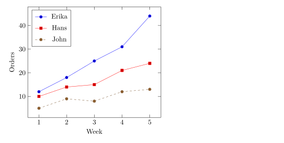
أنماط الخطوط والعلامات
تحدد الخيارات بعد \addplot اللون والخط والعلامات. ويمكنك الجمع بينها بحرية.
| الخيار | القيم | في Scissor LaTeX |
|---|---|---|
| اللون | red، blue!60!black، color=teal، أي اسم أو مزيج من xcolor | يعمل |
| سُمك الخط | ultra thin، very thin، thin، semithick، thick، very thick، ultra thick، line width=1.5pt | يعمل |
| نمط التقطيع | solid، dashed، dotted، densely dashed، loosely dotted، dashdotted، dash pattern=on 4pt off 2pt | يعمل |
mark= | *، o، square*، square، triangle*، triangle، diamond*، diamond، x، +، star، pentagon*، asterisk، otimes*، |، -، none | يعمل |
mark size=3pt | نصف قطر العلامة | يعمل |
mark options={fill=white} | نمط العلامات وحدها | يعمل |
mark repeat=2 | علامة على كل نقطة ثانية | يعمل |
no marks، only marks | خطوط فقط، علامات فقط | يعمل |
الألوان وأنماط التقطيع والعلامات
\begin{tikzpicture}
  \begin{axis}[domain=0:4, samples=9, legend pos=outer north east]
    \addplot[blue, thick, mark=*] {x};
    \addplot[red, dashed, mark=square*, mark options={fill=white}] {x^1.5/2};
    \addplot[teal, densely dotted, very thick] {sqrt(x)};
    \addplot[orange, mark=triangle*, mark size=3pt, only marks] {4 - x};
    \legend{linear, power, root, falling}
  \end{axis}
\end{tikzpicture}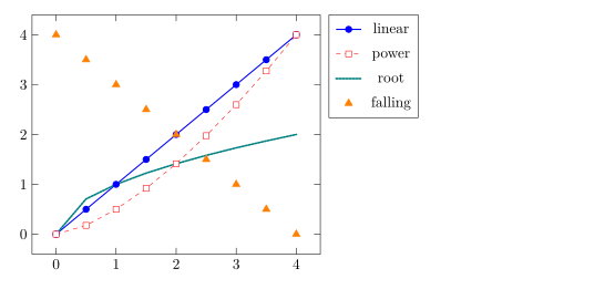
تُرسم العلامات دائمًا بخطوط متصلة، حتى على سلسلة متقطعة، كما في pgfplots.
اختيار قائمة أنماط دورية
قائمة الأنماط الدورية هي تسلسل الأنماط الذي تستخدمه أوامر \addplot البسيطة. اختر قائمة مدمجة باستخدام cycle list name، أو اكتب قائمتك الخاصة باستخدام cycle list.
قائمة black white الدورية، وقائمة مخصصة
\begin{tikzpicture}
  \begin{axis}[cycle list name=black white, width=6.5cm, height=5cm, title={black white}]
    \addplot coordinates {(0,0) (1,1) (2,4)};
    \addplot coordinates {(0,1) (1,2) (2,2)};
    \addplot coordinates {(0,2) (1,0) (2,1)};
  \end{axis}
\end{tikzpicture}
\begin{tikzpicture}
  \begin{axis}[cycle list={{red, thick}, {blue, dashed}}, width=6.5cm, height=5cm, title={custom}]
    \addplot coordinates {(0,0) (1,1) (2,4)};
    \addplot coordinates {(0,1) (1,2) (2,2)};
  \end{axis}
\end{tikzpicture}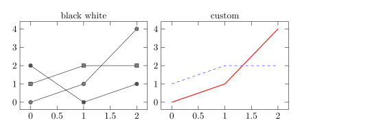
الأسماء المدمجة التي تعمل: color (الافتراضية)، وexotic، وblack white، وmark list، وlinestyles. ويعرّف \pgfplotscreateplotcyclelist{name}{...} في التمهيد قائمة يمكنك إعادة استخدامها.
المنحنيات الناعمة والدرجات
يرسم smooth منحنى يمر بالنقاط بدلًا من قطع مستقيمة؛ ويتحكم tension (الافتراضي 0.55) في مدى استدارته. ويرسم const plot دالة درجية تحتفظ بكل قيمة حتى النقطة التالية.
smooth وconst plot
\begin{tikzpicture}
  \begin{axis}[ymin=0, legend pos=north west]
    \addplot+[smooth] coordinates {(0,1) (1,2.5) (2,1.8) (3,3.2) (4,2.4)};
    \addplot+[const plot] coordinates {(0,0.5) (1,1) (2,1.5) (3,1.2) (4,2)};
    \legend{smooth, const plot}
  \end{axis}
\end{tikzpicture}
الدوال بالدرجات والراديان
تستخدم الصيغ pgfmath: + - * / ^ والأقواس وsqrt وexp وln وabs وmin وmax وsin وcos وtan وغيرها، مع pi وe ثابتين. الزوايا بالدرجات، لذا حوّل الراديان باستخدام deg(x).
sin وcos على مدى دورة واحدة
\begin{tikzpicture}
  \begin{axis}[domain=0:2*pi, samples=80, xlabel=$t$,
               xtick={0,1.5708,3.1416,4.7124,6.2832},
               xticklabels={$0$,$\frac{\pi}{2}$,$\pi$,$\frac{3\pi}{2}$,$2\pi$},
               legend pos=south west]
    \addplot[blue, thick] {sin(deg(x))};
    \addplot[red, thick, dashed] {cos(deg(x))};
    \legend{$\sin t$, $\cos t$}
  \end{axis}
\end{tikzpicture}
المنحنيات الوسيطية
لرسم منحنى معطى بـ x(t) وy(t)، اكتب الصيغتين بين قوسين، تفصل بينهما فاصلة، واضبط variable=t.
منحنى ليساجو
\begin{tikzpicture}
  \begin{axis}[axis lines=middle, xmin=-1.3, xmax=1.3, ymin=-1.3, ymax=1.3]
    \addplot[purple, thick, domain=0:360, samples=120, variable=t]
      ({cos(t)}, {sin(2*t)});
  \end{axis}
\end{tikzpicture}
فجوات في المنحنى
دالة مثل 1/x تنطلق نحو اللانهاية. يُسقط restrict y to domain النقاط الواقعة خارج نطاق ما، ويقطع unbounded coords=jump الخط هناك بدلًا من وصل الفرعين. ضع كليهما على \addplot.
1/x مع انقطاع عند الصفر
\begin{tikzpicture}
  \begin{axis}[ymin=-10, ymax=10, axis lines=middle]
    \addplot[blue, thick, domain=-3:3, samples=200,
             restrict y to domain=-10:10, unbounded coords=jump] {1/x};
  \end{axis}
\end{tikzpicture}
ما الذي يختلف عن تثبيت TeX
يصف دليل pgfplots على CTAN كل خيار: ctan.org/pkg/pgfplots. وللنقاط من دون خطوط، راجع رسوم النقاط المبعثرة.
راجع أيضًا أساسيات pgfplots والمحاور اللوغاريتمية ومجموعات الرسوم والبيانات من CSV.
أسئلة وأجوبة
كيف أرسم دالة في LaTeX؟
اكتب \addplot[domain=a:b, samples=n] {formula}; داخل axis، مستخدمًا x متغيرًا، مثل {x^2 - 1}.
كيف أزيل العلامات من خط؟
أضف no marks إلى خيارات \addplot، أو أعطِ خيارات من دون + (مثل \addplot[blue])، فيُرسم خط بسيط.
لماذا تبدو sin(x) مسطّحة تقريبًا؟
يقرأ pgfplots الزاوية بالدرجات، لذا فإن sin(x) على المدى من 0 إلى 6 لا يغطي إلا 6 درجات. اكتب sin(deg(x)).
كل مثال في هذه الصفحة ينضّده Scissor LaTeX عند بناء الموقع. آخر تحديث: 2026-11-07.