


pgfplots से लाइन प्लॉट
axis के अंदर हर लाइन के लिए एक \addplot जोड़ें; हर एक को red, dashed, thick या mark=square* जैसे ऑप्शन से स्टाइल दें, या साइकिल लिस्ट को आपके लिए स्टाइल चुनने दें।
एक ऐक्सिस में कई लाइनें
हर \addplot एक सीरीज़ जोड़ता है। ऑप्शन के बिना सीरीज़ बारी-बारी से साइकिल लिस्ट से अपनी स्टाइल लेती हैं। \addplot+[...] से आप वह स्टाइल रखते हैं और उसका एक हिस्सा बदलते हैं।
डिफ़ॉल्ट साइकिल लिस्ट से तीन सीरीज़
\begin{tikzpicture}
  \begin{axis}[xlabel=Week, ylabel=Orders, legend pos=north west]
    \addplot coordinates {(1,12) (2,18) (3,25) (4,31) (5,44)};
    \addplot coordinates {(1,10) (2,14) (3,15) (4,21) (5,24)};
    \addplot+[dashed] coordinates {(1,5) (2,9) (3,8) (4,12) (5,13)};
    \legend{Erika, Hans, John}
  \end{axis}
\end{tikzpicture}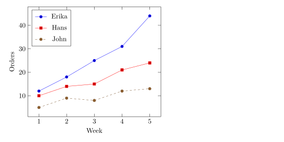
लाइन स्टाइल और मार्क
\addplot के बाद के ऑप्शन रंग, लाइन और मार्क तय करते हैं। आप इन्हें अपनी मर्ज़ी से मिला सकते हैं।
| ऑप्शन | वैल्यू | Scissor LaTeX में |
|---|---|---|
| रंग | red, blue!60!black, color=teal, कोई भी xcolor नाम या मिश्रण | काम करता है |
| लाइन की मोटाई | ultra thin, very thin, thin, semithick, thick, very thick, ultra thick, line width=1.5pt | काम करता है |
| डैश पैटर्न | solid, dashed, dotted, densely dashed, loosely dotted, dashdotted, dash pattern=on 4pt off 2pt | काम करता है |
mark= | *, o, square*, square, triangle*, triangle, diamond*, diamond, x, +, star, pentagon*, asterisk, otimes*, |, -, none | काम करता है |
mark size=3pt | मार्क की त्रिज्या | काम करता है |
mark options={fill=white} | सिर्फ़ मार्क की स्टाइल | काम करता है |
mark repeat=2 | हर दूसरे पॉइंट पर एक मार्क | काम करता है |
no marks, only marks | सिर्फ़ लाइनें, सिर्फ़ मार्क | काम करता है |
रंग, डैश पैटर्न और मार्क
\begin{tikzpicture}
  \begin{axis}[domain=0:4, samples=9, legend pos=outer north east]
    \addplot[blue, thick, mark=*] {x};
    \addplot[red, dashed, mark=square*, mark options={fill=white}] {x^1.5/2};
    \addplot[teal, densely dotted, very thick] {sqrt(x)};
    \addplot[orange, mark=triangle*, mark size=3pt, only marks] {4 - x};
    \legend{linear, power, root, falling}
  \end{axis}
\end{tikzpicture}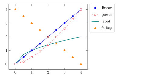
pgfplots की तरह, मार्क हमेशा सॉलिड लाइनों से ड्रॉ होते हैं, डैश्ड सीरीज़ पर भी।
साइकिल लिस्ट चुनना
साइकिल लिस्ट स्टाइल का वह क्रम है जिसे सादे \addplot कमांड इस्तेमाल करते हैं। cycle list name से कोई बिल्ट-इन लिस्ट चुनें, या cycle list से अपनी लिस्ट लिखें।
black white साइकिल लिस्ट, और एक कस्टम लिस्ट
\begin{tikzpicture}
  \begin{axis}[cycle list name=black white, width=6.5cm, height=5cm, title={black white}]
    \addplot coordinates {(0,0) (1,1) (2,4)};
    \addplot coordinates {(0,1) (1,2) (2,2)};
    \addplot coordinates {(0,2) (1,0) (2,1)};
  \end{axis}
\end{tikzpicture}
\begin{tikzpicture}
  \begin{axis}[cycle list={{red, thick}, {blue, dashed}}, width=6.5cm, height=5cm, title={custom}]
    \addplot coordinates {(0,0) (1,1) (2,4)};
    \addplot coordinates {(0,1) (1,2) (2,2)};
  \end{axis}
\end{tikzpicture}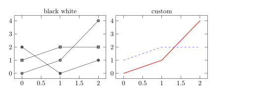
काम करने वाले बिल्ट-इन नाम: color (डिफ़ॉल्ट), exotic, black white, mark list और linestyles। प्रीएम्बल में \pgfplotscreateplotcyclelist{name}{...} एक ऐसी लिस्ट बनाता है जिसे आप दोबारा इस्तेमाल कर सकते हैं।
स्मूद कर्व और स्टेप
smooth सीधे टुकड़ों की जगह पॉइंट से होकर एक कर्व ड्रॉ करता है; tension (डिफ़ॉल्ट 0.55) तय करता है कि वह कितना गोल हो। const plot एक स्टेप फ़ंक्शन ड्रॉ करता है जो हर वैल्यू को अगले पॉइंट तक बनाए रखता है।
smooth और const plot
\begin{tikzpicture}
  \begin{axis}[ymin=0, legend pos=north west]
    \addplot+[smooth] coordinates {(0,1) (1,2.5) (2,1.8) (3,3.2) (4,2.4)};
    \addplot+[const plot] coordinates {(0,0.5) (1,1) (2,1.5) (3,1.2) (4,2)};
    \legend{smooth, const plot}
  \end{axis}
\end{tikzpicture}
डिग्री और रेडियन में फ़ंक्शन
फ़ॉर्मूले pgfmath इस्तेमाल करते हैं: + - * / ^, कोष्ठक, sqrt, exp, ln, abs, min, max, sin, cos, tan और भी, साथ में कॉन्स्टेंट के रूप में pi और e। कोण डिग्री में होते हैं, इसलिए रेडियन को deg(x) से बदलें।
एक पीरियड पर sin और cos
\begin{tikzpicture}
  \begin{axis}[domain=0:2*pi, samples=80, xlabel=$t$,
               xtick={0,1.5708,3.1416,4.7124,6.2832},
               xticklabels={$0$,$\frac{\pi}{2}$,$\pi$,$\frac{3\pi}{2}$,$2\pi$},
               legend pos=south west]
    \addplot[blue, thick] {sin(deg(x))};
    \addplot[red, thick, dashed] {cos(deg(x))};
    \legend{$\sin t$, $\cos t$}
  \end{axis}
\end{tikzpicture}
पैरामेट्रिक कर्व
x(t) और y(t) से दिए गए कर्व को प्लॉट करने के लिए दोनों फ़ॉर्मूले कोष्ठक में, कॉमा से अलग करके लिखें, और variable=t सेट करें।
एक Lissajous कर्व
\begin{tikzpicture}
  \begin{axis}[axis lines=middle, xmin=-1.3, xmax=1.3, ymin=-1.3, ymax=1.3]
    \addplot[purple, thick, domain=0:360, samples=120, variable=t]
      ({cos(t)}, {sin(2*t)});
  \end{axis}
\end{tikzpicture}
कर्व में गैप
1/x जैसा फ़ंक्शन अनंत की ओर भागता है। restrict y to domain किसी रेंज से बाहर के पॉइंट हटा देता है, और unbounded coords=jump दोनों शाखाओं को जोड़ने की जगह वहाँ लाइन तोड़ देता है। दोनों को \addplot पर लगाएँ।
शून्य पर ब्रेक के साथ 1/x
\begin{tikzpicture}
  \begin{axis}[ymin=-10, ymax=10, axis lines=middle]
    \addplot[blue, thick, domain=-3:3, samples=200,
             restrict y to domain=-10:10, unbounded coords=jump] {1/x};
  \end{axis}
\end{tikzpicture}
TeX इंस्टॉलेशन से क्या अलग है
CTAN पर pgfplots मैनुअल हर ऑप्शन के बारे में बताता है: ctan.org/pkg/pgfplots। बिना लाइनों वाले पॉइंट के लिए देखें स्कैटर प्लॉट।
यह भी देखें: pgfplots की बुनियादी बातें, लॉगरिदमिक ऐक्सिस, ग्रुप प्लॉट और CSV से डेटा।
सवाल और जवाब
LaTeX में फ़ंक्शन कैसे प्लॉट करें?
axis के अंदर \addplot[domain=a:b, samples=n] {formula}; लिखें, वेरिएबल के रूप में x इस्तेमाल करते हुए, जैसे {x^2 - 1}।
किसी लाइन से मार्क कैसे हटाएँ?
\addplot के ऑप्शन में no marks जोड़ें, या + के बिना ऑप्शन दें (जैसे \addplot[blue]), जो एक सादी लाइन ड्रॉ करता है।
sin(x) लगभग सपाट क्यों दिखता है?
pgfplots कोण को डिग्री में पढ़ता है, इसलिए 0 से 6 तक sin(x) सिर्फ़ 6 डिग्री कवर करता है। sin(deg(x)) लिखें।
इस पेज का हर उदाहरण साइट बनते समय Scissor LaTeX टाइपसेट करता है। पिछला अपडेट: 2026-11-07।