


pgfplots の折れ線グラフ
axis の中に線ごとに 1 つの \addplot を追加します。red、dashed、thick、mark=square* などのオプションでそれぞれのスタイルを指定するか、サイクルリストに選ばせます。
1 つの軸に複数の線
\addplot ごとに系列が 1 つ追加されます。オプションがなければ、系列は順にサイクルリストからスタイルを取ります。\addplot+[...] を使うと、そのスタイルを保ったまま一部だけを変えられます。
デフォルトのサイクルリストによる 3 つの系列
\begin{tikzpicture}
  \begin{axis}[xlabel=Week, ylabel=Orders, legend pos=north west]
    \addplot coordinates {(1,12) (2,18) (3,25) (4,31) (5,44)};
    \addplot coordinates {(1,10) (2,14) (3,15) (4,21) (5,24)};
    \addplot+[dashed] coordinates {(1,5) (2,9) (3,8) (4,12) (5,13)};
    \legend{Erika, Hans, John}
  \end{axis}
\end{tikzpicture}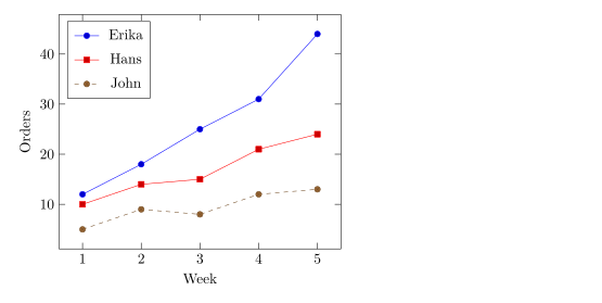
線のスタイルとマーカー
\addplot の後のオプションで、色、線、マーカーを指定します。これらは自由に組み合わせられます。
| オプション | 値 | Scissor LaTeX での対応 |
|---|---|---|
| 色 | red、blue!60!black、color=teal、xcolor の任意の色名や混色 | 使える |
| 線の太さ | ultra thin、very thin、thin、semithick、thick、very thick、ultra thick、line width=1.5pt | 使える |
| 破線のパターン | solid、dashed、dotted、densely dashed、loosely dotted、dashdotted、dash pattern=on 4pt off 2pt | 使える |
mark= | *、o、square*、square、triangle*、triangle、diamond*、diamond、x、+、star、pentagon*、asterisk、otimes*、|、-、none | 使える |
mark size=3pt | マーカーの半径 | 使える |
mark options={fill=white} | マーカーだけのスタイル | 使える |
mark repeat=2 | 1 点おきにマーカーを付ける | 使える |
no marks、only marks | 線だけ、マーカーだけ | 使える |
色、破線のパターン、マーカー
\begin{tikzpicture}
  \begin{axis}[domain=0:4, samples=9, legend pos=outer north east]
    \addplot[blue, thick, mark=*] {x};
    \addplot[red, dashed, mark=square*, mark options={fill=white}] {x^1.5/2};
    \addplot[teal, densely dotted, very thick] {sqrt(x)};
    \addplot[orange, mark=triangle*, mark size=3pt, only marks] {4 - x};
    \legend{linear, power, root, falling}
  \end{axis}
\end{tikzpicture}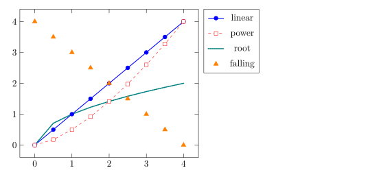
pgfplots と同じく、マーカーは破線の系列でも常に実線で描かれます。
サイクルリストを選ぶ
サイクルリストとは、オプションなしの \addplot が順に使うスタイルの並びです。組み込みのものは cycle list name で選び、独自のものは cycle list で書きます。
black white のサイクルリストと独自のリスト
\begin{tikzpicture}
  \begin{axis}[cycle list name=black white, width=6.5cm, height=5cm, title={black white}]
    \addplot coordinates {(0,0) (1,1) (2,4)};
    \addplot coordinates {(0,1) (1,2) (2,2)};
    \addplot coordinates {(0,2) (1,0) (2,1)};
  \end{axis}
\end{tikzpicture}
\begin{tikzpicture}
  \begin{axis}[cycle list={{red, thick}, {blue, dashed}}, width=6.5cm, height=5cm, title={custom}]
    \addplot coordinates {(0,0) (1,1) (2,4)};
    \addplot coordinates {(0,1) (1,2) (2,2)};
  \end{axis}
\end{tikzpicture}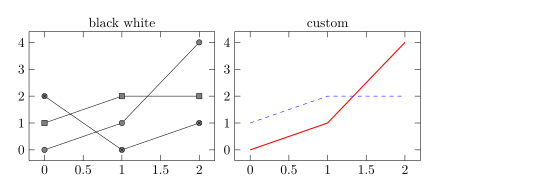
使える組み込みの名前は、color(デフォルト)、exotic、black white、mark list、linestyles です。プリアンブルで \pgfplotscreateplotcyclelist{name}{...} と書くと、使い回せるリストを定義できます。
なめらかな曲線と階段
smooth は、直線の線分の代わりに点を通る曲線を描きます。丸みは tension(デフォルトは 0.55)で調整します。const plot は、次の点まで各値を保つ階段関数を描きます。
smooth と const plot
\begin{tikzpicture}
  \begin{axis}[ymin=0, legend pos=north west]
    \addplot+[smooth] coordinates {(0,1) (1,2.5) (2,1.8) (3,3.2) (4,2.4)};
    \addplot+[const plot] coordinates {(0,0.5) (1,1) (2,1.5) (3,1.2) (4,2)};
    \legend{smooth, const plot}
  \end{axis}
\end{tikzpicture}
度とラジアンの関数
数式には pgfmath を使います。+ - * / ^、かっこ、sqrt、exp、ln、abs、min、max、sin、cos、tan などがあり、定数として pi と e を使えます。角度は度で計算されるので、ラジアンは deg(x) で変換します。
1 周期分の sin と cos
\begin{tikzpicture}
  \begin{axis}[domain=0:2*pi, samples=80, xlabel=$t$,
               xtick={0,1.5708,3.1416,4.7124,6.2832},
               xticklabels={$0$,$\frac{\pi}{2}$,$\pi$,$\frac{3\pi}{2}$,$2\pi$},
               legend pos=south west]
    \addplot[blue, thick] {sin(deg(x))};
    \addplot[red, thick, dashed] {cos(deg(x))};
    \legend{$\sin t$, $\cos t$}
  \end{axis}
\end{tikzpicture}
媒介変数表示の曲線
x(t) と y(t) で与えられる曲線をプロットするには、両方の数式をかっこの中にカンマで区切って書き、variable=t を指定します。
リサージュ曲線
\begin{tikzpicture}
  \begin{axis}[axis lines=middle, xmin=-1.3, xmax=1.3, ymin=-1.3, ymax=1.3]
    \addplot[purple, thick, domain=0:360, samples=120, variable=t]
      ({cos(t)}, {sin(2*t)});
  \end{axis}
\end{tikzpicture}
曲線の切れ目
1/x のような関数は無限大に発散します。restrict y to domain は範囲外の点を取り除き、unbounded coords=jump は 2 つの枝を結ばずにそこで線を切ります。どちらも \addplot に指定します。
0 で切れ目を入れた 1/x
\begin{tikzpicture}
  \begin{axis}[ymin=-10, ymax=10, axis lines=middle]
    \addplot[blue, thick, domain=-3:3, samples=200,
             restrict y to domain=-10:10, unbounded coords=jump] {1/x};
  \end{axis}
\end{tikzpicture}
TeX のインストール環境との違い
すべてのオプションは CTAN の pgfplots のマニュアルで説明されています:ctan.org/pkg/pgfplots。線なしの点については散布図をご覧ください。
pgfplots の基本、対数軸、グループプロット、CSV のデータもご覧ください。
よくある質問
LaTeX で関数をプロットするにはどうすればよいですか?
axis の中に \addplot[domain=a:b, samples=n] {formula}; と書き、変数には x を使います。たとえば {x^2 - 1} です。
線からマーカーを消すにはどうすればよいですか?
\addplot のオプションに no marks を追加するか、+ なしでオプションを指定します(たとえば \addplot[blue])。そうすると単なる線が描かれます。
sin(x) がほとんど平らに見えるのはなぜですか?
pgfplots は角度を度として読むので、0 から 6 の sin(x) は 6 度分しかありません。sin(deg(x)) と書いてください。
このページの例はすべて、サイトのビルド時に Scissor LaTeX で組版されています。 最終更新:2026-11-07