


กราฟเส้นด้วย pgfplots
ใส่ \addplot หนึ่งคำสั่งต่อหนึ่งเส้นภายใน axis แล้วกำหนดสไตล์แต่ละเส้นด้วยตัวเลือกอย่าง red, dashed, thick หรือ mark=square* หรือปล่อยให้ cycle list เลือกสไตล์ให้
หลายเส้นในแกนเดียว
\addplot แต่ละคำสั่งเพิ่มข้อมูลหนึ่งชุด หากไม่ใส่ตัวเลือก ข้อมูลแต่ละชุดจะได้สไตล์จาก cycle list ตามลำดับ ส่วน \addplot+[...] จะคงสไตล์นั้นไว้และเปลี่ยนเพียงบางส่วน
ข้อมูลสามชุดจาก cycle list เริ่มต้น
\begin{tikzpicture}
  \begin{axis}[xlabel=Week, ylabel=Orders, legend pos=north west]
    \addplot coordinates {(1,12) (2,18) (3,25) (4,31) (5,44)};
    \addplot coordinates {(1,10) (2,14) (3,15) (4,21) (5,24)};
    \addplot+[dashed] coordinates {(1,5) (2,9) (3,8) (4,12) (5,13)};
    \legend{Erika, Hans, John}
  \end{axis}
\end{tikzpicture}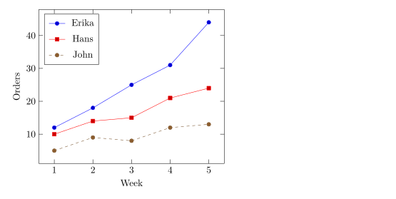
สไตล์เส้นและเครื่องหมายจุด
ตัวเลือกหลัง \addplot กำหนดสี เส้น และเครื่องหมายจุด คุณผสมตัวเลือกเหล่านี้ได้อย่างอิสระ
| ตัวเลือก | ค่า | ใน Scissor LaTeX |
|---|---|---|
| สี | red, blue!60!black, color=teal, ชื่อสีหรือสีผสมใดก็ได้ของ xcolor | ใช้ได้ |
| ความหนาเส้น | ultra thin, very thin, thin, semithick, thick, very thick, ultra thick, line width=1.5pt | ใช้ได้ |
| รูปแบบเส้นประ | solid, dashed, dotted, densely dashed, loosely dotted, dashdotted, dash pattern=on 4pt off 2pt | ใช้ได้ |
mark= | *, o, square*, square, triangle*, triangle, diamond*, diamond, x, +, star, pentagon*, asterisk, otimes*, |, -, none | ใช้ได้ |
mark size=3pt | รัศมีของเครื่องหมายจุด | ใช้ได้ |
mark options={fill=white} | สไตล์ของเครื่องหมายจุดเท่านั้น | ใช้ได้ |
mark repeat=2 | เครื่องหมายทุก ๆ จุดที่สอง | ใช้ได้ |
no marks, only marks | เส้นอย่างเดียว, เครื่องหมายจุดอย่างเดียว | ใช้ได้ |
สี รูปแบบเส้นประ และเครื่องหมายจุด
\begin{tikzpicture}
  \begin{axis}[domain=0:4, samples=9, legend pos=outer north east]
    \addplot[blue, thick, mark=*] {x};
    \addplot[red, dashed, mark=square*, mark options={fill=white}] {x^1.5/2};
    \addplot[teal, densely dotted, very thick] {sqrt(x)};
    \addplot[orange, mark=triangle*, mark size=3pt, only marks] {4 - x};
    \legend{linear, power, root, falling}
  \end{axis}
\end{tikzpicture}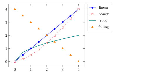
เครื่องหมายจุดจะวาดด้วยเส้นทึบเสมอ แม้อยู่บนข้อมูลชุดที่เป็นเส้นประ เหมือนใน pgfplots
การเลือก cycle list
cycle list คือลำดับสไตล์ที่คำสั่ง \addplot แบบไม่มีตัวเลือกใช้ เลือกชุดที่มีมาให้ด้วย cycle list name หรือเขียนชุดของคุณเองด้วย cycle list
cycle list แบบ black white และแบบกำหนดเอง
\begin{tikzpicture}
  \begin{axis}[cycle list name=black white, width=6.5cm, height=5cm, title={black white}]
    \addplot coordinates {(0,0) (1,1) (2,4)};
    \addplot coordinates {(0,1) (1,2) (2,2)};
    \addplot coordinates {(0,2) (1,0) (2,1)};
  \end{axis}
\end{tikzpicture}
\begin{tikzpicture}
  \begin{axis}[cycle list={{red, thick}, {blue, dashed}}, width=6.5cm, height=5cm, title={custom}]
    \addplot coordinates {(0,0) (1,1) (2,4)};
    \addplot coordinates {(0,1) (1,2) (2,2)};
  \end{axis}
\end{tikzpicture}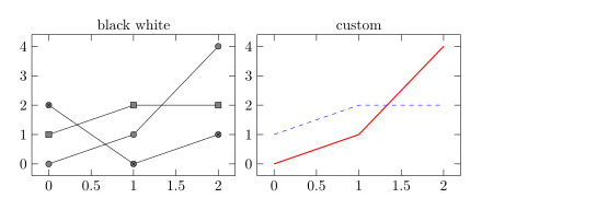
ชื่อชุดที่มีมาให้และใช้ได้ ได้แก่ color (ค่าเริ่มต้น), exotic, black white, mark list และ linestyles ส่วน \pgfplotscreateplotcyclelist{name}{...} ในส่วนนำของเอกสารจะกำหนดชุดที่คุณนำกลับมาใช้ซ้ำได้
เส้นโค้งเรียบและขั้นบันได
smooth วาดเส้นโค้งผ่านจุดต่าง ๆ แทนการต่อด้วยเส้นตรง โดย tension (ค่าเริ่มต้น 0.55) ควบคุมความโค้งมน ส่วน const plot วาดฟังก์ชันขั้นบันไดที่คงค่าแต่ละค่าไว้จนถึงจุดถัดไป
smooth และ const plot
\begin{tikzpicture}
  \begin{axis}[ymin=0, legend pos=north west]
    \addplot+[smooth] coordinates {(0,1) (1,2.5) (2,1.8) (3,3.2) (4,2.4)};
    \addplot+[const plot] coordinates {(0,0.5) (1,1) (2,1.5) (3,1.2) (4,2)};
    \legend{smooth, const plot}
  \end{axis}
\end{tikzpicture}
ฟังก์ชันในหน่วยองศาและเรเดียน
สูตรใช้ pgfmath ได้แก่ + - * / ^ วงเล็บ sqrt, exp, ln, abs, min, max, sin, cos, tan และอื่น ๆ โดยมี pi และ e เป็นค่าคงที่ มุมอยู่ในหน่วยองศา จึงต้องแปลงเรเดียนด้วย deg(x)
sin และ cos ในหนึ่งคาบ
\begin{tikzpicture}
  \begin{axis}[domain=0:2*pi, samples=80, xlabel=$t$,
               xtick={0,1.5708,3.1416,4.7124,6.2832},
               xticklabels={$0$,$\frac{\pi}{2}$,$\pi$,$\frac{3\pi}{2}$,$2\pi$},
               legend pos=south west]
    \addplot[blue, thick] {sin(deg(x))};
    \addplot[red, thick, dashed] {cos(deg(x))};
    \legend{$\sin t$, $\cos t$}
  \end{axis}
\end{tikzpicture}
เส้นโค้งอิงพารามิเตอร์
หากต้องการวาดเส้นโค้งที่กำหนดด้วย x(t) และ y(t) ให้เขียนสูตรทั้งสองในวงเล็บ คั่นด้วยจุลภาค และตั้งค่า variable=t
เส้นโค้งลิสซาจู
\begin{tikzpicture}
  \begin{axis}[axis lines=middle, xmin=-1.3, xmax=1.3, ymin=-1.3, ymax=1.3]
    \addplot[purple, thick, domain=0:360, samples=120, variable=t]
      ({cos(t)}, {sin(2*t)});
  \end{axis}
\end{tikzpicture}
ช่วงขาดในเส้นโค้ง
ฟังก์ชันอย่าง 1/x พุ่งไปสู่อนันต์ restrict y to domain จะตัดจุดที่อยู่นอกช่วงออก และ unbounded coords=jump จะตัดเส้นตรงนั้นแทนการเชื่อมสองกิ่งเข้าด้วยกัน ให้ใส่ทั้งสองตัวเลือกไว้ที่ \addplot
1/x ที่ขาดตอนที่ศูนย์
\begin{tikzpicture}
  \begin{axis}[ymin=-10, ymax=10, axis lines=middle]
    \addplot[blue, thick, domain=-3:3, samples=200,
             restrict y to domain=-10:10, unbounded coords=jump] {1/x};
  \end{axis}
\end{tikzpicture}
สิ่งที่ต่างจากการติดตั้ง TeX
คู่มือ pgfplots บน CTAN อธิบายตัวเลือกทุกตัว: ctan.org/pkg/pgfplots สำหรับจุดที่ไม่มีเส้น ดูแผนภาพการกระจาย
ดูเพิ่มเติม พื้นฐาน pgfplots, แกนลอการิทึม, กราฟแบบกลุ่ม และ ข้อมูลจาก CSV
คำถามและคำตอบ
จะวาดกราฟฟังก์ชันใน LaTeX ได้อย่างไร
เขียน \addplot[domain=a:b, samples=n] {formula}; ภายใน axis โดยใช้ x เป็นตัวแปร เช่น {x^2 - 1}
จะเอาเครื่องหมายจุดออกจากเส้นได้อย่างไร
เพิ่ม no marks ในตัวเลือกของ \addplot หรือใส่ตัวเลือกโดยไม่มี + (เช่น \addplot[blue]) ซึ่งจะวาดเส้นเปล่า
ทำไม sin(x) ดูเกือบแบน
pgfplots อ่านมุมเป็นองศา ดังนั้น sin(x) บนช่วง 0 ถึง 6 จึงครอบคลุมเพียง 6 องศา ให้เขียน sin(deg(x))
ทุกตัวอย่างในหน้านี้จัดหน้าโดย Scissor LaTeX ขณะสร้างเว็บไซต์ อัปเดตล่าสุด 2026-11-07