


Contours, heat maps and colour maps
Use \addplot3 in an axis with view={0}{90}: surf or matrix plot for a heat map, contour filled for filled contours, and add colorbar and a colormap for the scale.
A heat map of a function
\addplot3 plots a function of x and y. Seen from above (view={0}{90}), a surf plot becomes a heat map: each cell is coloured by its value through the colour map. shader=interp blends the colours smoothly; shader=flat gives one colour per cell.
A smooth heat map with a colour bar
\begin{tikzpicture}
  \begin{axis}[view={0}{90}, colorbar, colormap/viridis,
               xlabel=$x$, ylabel=$y$, enlargelimits=false]
    \addplot3[surf, shader=interp, domain=-2:2, y domain=-2:2, samples=30]
      {exp(-x^2 - y^2) * (1 + x)};
  \end{axis}
\end{tikzpicture}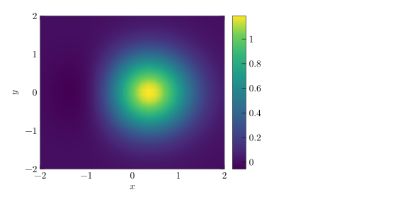
domain sets the range of x, y domain the range of y, and samples the grid size (25 by default, samples y for a different count in y).
Filled contours
contour filled divides the values into bands. number= sets how many contour levels there are; levels={...} lists them yourself.
Filled contours of a two-peak function
\begin{tikzpicture}
  \begin{axis}[view={0}{90}, colorbar, colormap/hot, enlargelimits=false]
    \addplot3[contour filled={number=8}, domain=-3:3, y domain=-3:3, samples=40]
      {exp(-(x-1)^2 - y^2) + 0.7*exp(-(x+1.2)^2 - (y-1)^2)};
  \end{axis}
\end{tikzpicture}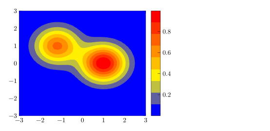
Heat map from a table: matrix plot
For measured data on a grid, matrix plot* draws one cell per row of a table. mesh/cols says how many columns the grid has, and point meta=explicit with meta= names the value column.
A 3 by 3 grid of values
\begin{tikzpicture}
  \begin{axis}[colorbar, colormap/bluered, enlargelimits=false,
               xtick=data, ytick=data, width=6.5cm, height=6cm]
    \addplot[matrix plot*, mesh/cols=3, point meta=explicit]
      table[meta=v] {
        x y v
        0 0 1
        1 0 4
        2 0 2
        0 1 3
        1 1 9
        2 1 5
        0 2 2
        1 2 6
        2 2 44
      };
  \end{axis}
\end{tikzpicture}
Contour lines
Lines without filling need contour levels computed for you. In pgfplots that is contour gnuplot or contour lua, which need extra programs or LuaLaTeX in a TeX installation. Scissor LaTeX computes the lines itself and draws them, and reminds you in the Problems tab that the code may not compile elsewhere.
Contour lines with contour gnuplot
\begin{tikzpicture}
  \begin{axis}[view={0}{90}, xlabel=$x$, ylabel=$y$]
    \addplot3[contour gnuplot={levels={0.2, 0.5, 0.8}},
              domain=-2:2, y domain=-2:2, samples=30]
      {exp(-x^2 - y^2)};
  \end{axis}
\end{tikzpicture}
Problems tab: contour gnuplot needs gnuplot and shell escape in LaTeX; contour filled or contour prepared compile everywhere
For a file that compiles everywhere, use contour filled, or contour prepared with precomputed contour data.
Colour maps and colour bars
| Option | What it does | In Scissor LaTeX |
|---|---|---|
colormap/viridis, /hot, /cool, /jet, /blackwhite, /bluered | built-in colour maps | Works |
colormap name=viridis | select a map by name | Works |
colormap={name}{rgb255=(..) rgb255=(..)} | your own map | Works |
colorbar, colorbar horizontal | a scale next to or under the plot | Works |
colorbar style={..} | ticks and labels of the colour bar | Works |
point meta min, point meta max | fix the colour range | Works |
shader=flat, shader=interp, shader=faceted | how cells are coloured | Works |
A custom colour map and a horizontal colour bar
\begin{tikzpicture}
  \begin{axis}[view={0}{90}, enlargelimits=false,
               colormap={sea}{rgb255=(255,255,255) rgb255=(120,180,220) rgb255=(10,40,100)},
               colorbar horizontal, width=7cm, height=6cm]
    \addplot3[surf, shader=flat, domain=0:2, y domain=0:2, samples=12] {x*y};
  \end{axis}
\end{tikzpicture}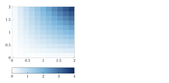
3D views
Scissor LaTeX draws \addplot3 only as seen from straight above. Any other view, including the default 3D view, leaves the axis empty and shows a message.
A 3D view is not drawn
\begin{tikzpicture}
  \begin{axis}[width=6cm, height=5cm]
    \addplot3[surf, domain=-2:2, y domain=-2:2] {x^2 - y^2};
  \end{axis}
\end{tikzpicture}
Problems tab: 3D plots are drawn only when seen from above (view={0}{90}) for now
What differs from a TeX installation
The pgfplots manual covers \addplot3, colour maps and contours in detail: ctan.org/pkg/pgfplots.
See also pgfplots basics, Logarithmic axes and pgfplots.
Questions and answers
How do I make a heat map in LaTeX?
Use \addplot3[surf, shader=interp] {f(x,y)}; (or matrix plot* for table data) in an axis with view={0}{90}, and add colorbar.
Does Scissor LaTeX draw 3D surface plots?
Not yet. \addplot3 is drawn only when seen from above (view={0}{90}); other views leave the axis empty and the Problems tab says so.
Why does contour gnuplot show a warning?
In a TeX installation it needs gnuplot and shell escape. Scissor LaTeX draws the contours anyway, but warns that the code may not compile elsewhere. contour filled compiles everywhere.
Every example on this page is typeset by Scissor LaTeX when the site is built. Last updated 2026-11-06.