


pgfplots basics: plots in LaTeX with examples
Load pgfplots, open a tikzpicture with an axis inside, and add each data series with \addplot, either as a list of coordinates or as a formula.
The smallest plot
Every pgfplots plot has the same three layers: a tikzpicture, an axis inside it, and one \addplot per data series. Load the package with \usepackage{pgfplots} in the preamble.
Four points joined by a line
\begin{tikzpicture}
  \begin{axis}
    \addplot coordinates {(0,1) (1,3) (2,2) (3,4)};
  \end{axis}
\end{tikzpicture}
The axis picks its own range and ticks from the data. A plain \addplot takes its colour and mark from the default cycle list: blue with round marks for the first series, red with squares for the second, and so on.
Plotting a formula
Instead of coordinates, give \addplot a formula in braces. domain sets the range of x and samples the number of points. Without them, pgfplots uses the range -5 to 5 with 25 samples.
A function with domain and samples
\begin{tikzpicture}
  \begin{axis}
    \addplot[blue, thick, domain=-2:2, samples=60] {x^3 - 2*x};
  \end{axis}
\end{tikzpicture}
Options in square brackets after \addplot style that series. When you give options without a +, the series is drawn in black (or the colour you name) without marks; \addplot+[...] keeps the cycle list style and adds your options to it.
Labels, title, legend and grid
These options go on the axis, so they affect the whole plot.
Axis labels, a title, a legend and a grid
\begin{tikzpicture}
  \begin{axis}[
      title={Cooling of a cup of tea},
      xlabel={Time (min)},
      ylabel={Temperature ($^\circ$C)},
      grid=major,
      legend pos=north east,
    ]
    \addplot coordinates {(0,80) (5,64) (10,53) (15,44) (20,38)};
    \addlegendentry{Measured}
    \addplot[red, domain=0:20, samples=40] {22 + 58*exp(-0.08*x)};
    \addlegendentry{Model}
  \end{axis}
\end{tikzpicture}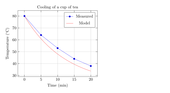
Labels are text, so math goes between $ ... $ as in a paragraph. \addlegendentry after each \addplot names that series; you can also list all names at the end with \legend{Measured, Model}.
Common axis options
| Option | What it does | In Scissor LaTeX |
|---|---|---|
xlabel, ylabel, title | text along the axes and above the plot | Works |
xmin, xmax, ymin, ymax | fix the visible range | Works |
width, height | size of the whole picture, for example width=\linewidth | Works |
grid=major, grid=both | grid lines at the major (and minor) ticks | Works |
xtick={0,1,2}, xticklabels={a,b,c} | choose the ticks and their labels | Works |
legend pos=north west | north west, north east, south west, south east, outer north east | Works |
axis lines=left | an L-shaped pair of axes with arrows instead of a box | Works (also middle, center, none) |
enlargelimits=false | no extra space around the data | Works |
axis equal | the same scale on both axes | Not supported yet: ignored with a message in the Problems tab |
Most other options from the pgfplots manual work as well; the line plots page lists styles and marks. An option the renderer does not know is ignored, and the Problems tab names it.
Size and placement
By default a plot is about 240 by 207 points, the pgfplots default. Set width and height on the axis to change it. To give a plot a caption and a number, put the tikzpicture inside a figure, as you would an image.
A plot in a figure with a caption
\begin{figure}[h]
  \centering
  \begin{tikzpicture}
    \begin{axis}[width=7cm, height=4.5cm, xlabel=$x$, ylabel=$x^2$]
      \addplot[domain=0:2, samples=30] {x^2};
    \end{axis}
  \end{tikzpicture}
  \caption{A parabola on $[0, 2]$.}
  \label{fig:parabola}
\end{figure}

Figure~\ref{fig:parabola} shows the parabola.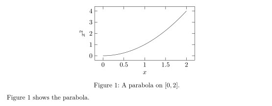
\resizebox{0.5\linewidth}{!}{...} around a single tikzpicture also works: the picture is scaled to that width.
What differs from a TeX installation
Everything on this page also compiles in a TeX installation with pgfplots. The full manual is on CTAN: ctan.org/pkg/pgfplots.
Questions and answers
Do I need to install pgfplots?
No. Write \usepackage{pgfplots} as usual. Scissor LaTeX recognises the package and draws the plots itself, in the browser.
Why is my function plot jagged?
pgfplots joins 25 points by default. Add samples=100 (or more) to the \addplot or the axis for a smoother curve, or add smooth to draw a curve through the points.
Can I use pgfplots without tikzpicture?
No, in LaTeX the axis environment always sits inside a tikzpicture. Scissor LaTeX follows the same rule, so your code also compiles elsewhere.
Every example on this page is typeset by Scissor LaTeX when the site is built. Last updated 2026-11-06.