


pgfplots の誤差棒
\addplot のオプションに error bars/.cd, y dir=both, y explicit を追加し、各点の後に +- (0, error) と誤差を書くか、y error= で表の列から誤差を読み込みます。
点と一緒に書く誤差
誤差棒は \addplot ごとにオンにします。error bars/.cd の後のキーで、描く方向と値の取得元を指定します。y explicit を使うと、各点が +- の後に自分の誤差を持ちます。
座標から読む対称な y の誤差
\begin{tikzpicture}
  \begin{axis}[xlabel={Length (m)}, ylabel={Period (s)}]
    \addplot+[error bars/.cd, y dir=both, y explicit]
      coordinates {
        (0.2,0.90) +- (0,0.05)
        (0.4,1.27) +- (0,0.04)
        (0.6,1.55) +- (0,0.06)
        (0.8,1.80) +- (0,0.05)
        (1.0,2.01) +- (0,0.07)
      };
  \end{axis}
\end{tikzpicture}
+- (ex, ey) では、1 つ目の数値が x の誤差、2 つ目が y の誤差です。描かれるのはオンにした方向だけです。
表の列から読む誤差
データが表の場合は、y error= で誤差の列を指定します。ファイルでも同じで、たとえば table[x=t, y=v, y error=dv, col sep=comma] {data.csv} と書きます。
列から読む y の誤差
\begin{tikzpicture}
  \begin{axis}[xlabel={Dose}, ylabel={Response}, ymin=0]
    \addplot+[only marks, error bars/.cd, y dir=both, y explicit]
      table[x=dose, y=mean, y error=sd] {
        dose mean sd
        1    2.1  0.3
        2    3.4  0.4
        4    5.0  0.6
        8    6.2  0.5
      };
  \end{axis}
\end{tikzpicture}
片側の誤差と固定の誤差
y dir=plus や y dir=minus は、上半分または下半分だけを描きます。明示的な値の代わりに、y fixed=0.2 ですべての点に同じ誤差を、y fixed relative=0.1 で値の 10% の誤差を付けられます。
上側だけの誤差と相対誤差
\begin{tikzpicture}
  \begin{axis}[ymin=0, legend pos=north west]
    \addplot+[error bars/.cd, y dir=plus, y fixed=0.4]
      coordinates {(1,2) (2,3) (3,3.5) (4,4.4)};
    \addplot+[error bars/.cd, y dir=both, y fixed relative=0.1]
      coordinates {(1,1) (2,1.6) (3,2.2) (4,2.5)};
    \legend{fixed $\pm 0.4$ (upper), relative 10\%}
  \end{axis}
\end{tikzpicture}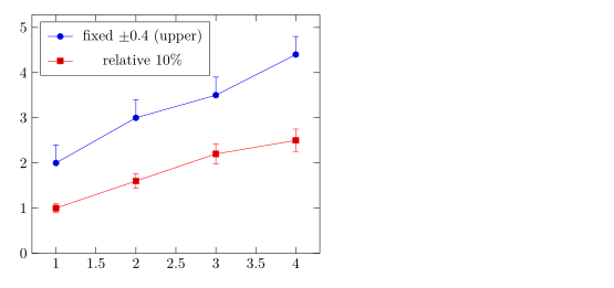
上下で異なる誤差
上側の誤差は += (0, up)、下側の誤差は -= (0, down) と書きます。
非対称な誤差
\begin{tikzpicture}
  \begin{axis}[width=7cm, height=5cm, xmin=0.5, xmax=3.5]
    \addplot+[only marks, error bars/.cd, y dir=both, y explicit]
      coordinates {
        (1,2.0) += (0,0.5) -= (0,0.1)
        (2,3.0) += (0,0.2) -= (0,0.6)
        (3,2.6) += (0,0.3) -= (0,0.3)
      };
  \end{axis}
\end{tikzpicture}
x と y の誤差
x dir と y dir で両方向をオンにします。error bar style で誤差棒のスタイルを指定します。
両方向の誤差棒
\begin{tikzpicture}
  \begin{axis}[xlabel=$x$, ylabel=$y$]
    \addplot+[only marks, mark=square*,
              error bars/.cd,
                x dir=both, x explicit,
                y dir=both, y explicit,
                error bar style={red, thick}]
      coordinates {
        (1.0,1.2) +- (0.15,0.20)
        (2.0,2.1) +- (0.20,0.15)
        (3.0,2.8) +- (0.10,0.30)
      };
  \end{axis}
\end{tikzpicture}
fill between による誤差の帯
連続した不確かさを示すには、上側と下側の曲線の間に網掛けをします。fillbetween ライブラリを読み込み、両方の曲線に name path で名前を付け、その間を塗ります。
曲線の周りの網掛けの帯
\documentclass{article}
\usepackage{pgfplots}
\usepgfplotslibrary{fillbetween}
\begin{document}
\begin{tikzpicture}
  \begin{axis}[domain=0:4, samples=40, xlabel=$t$, ylabel=$y$]
    \addplot[name path=upper, draw=none] {exp(-0.5*x) + 0.1 + 0.05*x};
    \addplot[name path=lower, draw=none] {exp(-0.5*x) - 0.1 - 0.05*x};
    \addplot[blue!20] fill between[of=upper and lower];
    \addplot[blue, thick] {exp(-0.5*x)};
  \end{axis}
\end{tikzpicture}
\end{document}
誤差棒のオプション
| オプション | 働き | Scissor LaTeX での対応 |
|---|---|---|
y dir=both、plus、minus、none | 誤差棒のどちら側を描くか(x dir も同様) | 使える |
y explicit、x explicit | 座標の +- または表の列から読む誤差 | 使える |
y error=col、x error=col、y error index=n | 誤差の入った表の列 | 使える |
+= (ex,ey)、-= (ex,ey) | 座標での上側と下側の個別の誤差 | 使える |
y fixed=v、y fixed relative=r | すべての点に同じ誤差 | 使える |
error bar style={..} | 誤差棒の色と線の太さ | 使える |
error mark=..、error mark options={..} | 両端のキャップ | 受け付けるが、キャップは常に短い線 |
TeX のインストール環境との違い
誤差棒は pgfplots のマニュアルの誤差棒の節で説明されています:ctan.org/pkg/pgfplots。
よくある質問
pgfplots で誤差棒を付けるにはどうすればよいですか?
\addplot+[error bars/.cd, y dir=both, y explicit] coordinates {(1,2) +- (0,0.3) ...}; と書きます。+- の後の 2 つ目の数値が y の誤差です。
CSV ファイルから誤差棒を読み込むにはどうすればよいですか?
表のオプションに y error=column を追加し、誤差棒のオプションに y explicit を指定します:table[x=a, y=b, y error=c, col sep=comma] {file.csv}。
誤差棒を上下で異なる長さにできますか?
はい。点の後に +- の代わりに += (0, up) と -= (0, down) を書きます。たとえば (1,2) += (0,0.5) -= (0,0.1) です。
このページの例はすべて、サイトのビルド時に Scissor LaTeX で組版されています。 最終更新:2026-11-07