


等高線、ヒートマップ、カラーマップ
view={0}{90} を指定した軸で \addplot3 を使います。ヒートマップには surf か matrix plot、塗りつぶした等高線には contour filled を使い、目盛りには colorbar と colormap を追加します。
関数のヒートマップ
\addplot3 は x と y の関数をプロットします。真上から見る(view={0}{90})と、surf のプロットはヒートマップになり、各セルが値に応じてカラーマップで色付けされます。shader=interp は色をなめらかにつなぎ、shader=flat はセルごとに 1 色にします。
カラーバー付きのなめらかなヒートマップ
\begin{tikzpicture}
  \begin{axis}[view={0}{90}, colorbar, colormap/viridis,
               xlabel=$x$, ylabel=$y$, enlargelimits=false]
    \addplot3[surf, shader=interp, domain=-2:2, y domain=-2:2, samples=30]
      {exp(-x^2 - y^2) * (1 + x)};
  \end{axis}
\end{tikzpicture}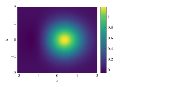
domain で x の範囲を、y domain で y の範囲を、samples で格子の大きさ(デフォルトは 25、y の数を変えるには samples y)を指定します。
塗りつぶした等高線
contour filled は値を帯に分けます。number= で等高線の段階の数を指定し、levels={...} で自分で段階を並べることもできます。
2 つの山を持つ関数の塗りつぶした等高線
\begin{tikzpicture}
  \begin{axis}[view={0}{90}, colorbar, colormap/hot, enlargelimits=false]
    \addplot3[contour filled={number=8}, domain=-3:3, y domain=-3:3, samples=40]
      {exp(-(x-1)^2 - y^2) + 0.7*exp(-(x+1.2)^2 - (y-1)^2)};
  \end{axis}
\end{tikzpicture}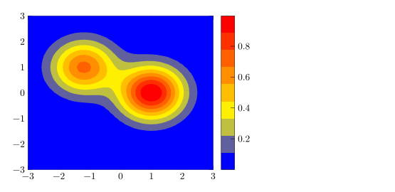
表から作るヒートマップ:matrix plot
格子上の測定データには、matrix plot* を使うと表の 1 行ごとに 1 つのセルが描かれます。mesh/cols で格子の列数を指定し、point meta=explicit と meta= で値の列を指定します。
3 × 3 の値の格子
\begin{tikzpicture}
  \begin{axis}[colorbar, colormap/bluered, enlargelimits=false,
               xtick=data, ytick=data, width=6.5cm, height=6cm]
    \addplot[matrix plot*, mesh/cols=3, point meta=explicit]
      table[meta=v] {
        x y v
        0 0 1
        1 0 4
        2 0 2
        0 1 3
        1 1 9
        2 1 5
        0 2 2
        1 2 6
        2 2 44
      };
  \end{axis}
\end{tikzpicture}
等高線
塗りつぶしのない線を描くには、等高線の段階を計算する必要があります。pgfplots では contour gnuplot か contour lua を使いますが、TeX のインストール環境では追加のプログラムか LuaLaTeX が必要です。Scissor LaTeX は線を自分で計算して描き、そのコードがほかの環境ではコンパイルできない可能性があることを「問題」タブで知らせます。
contour gnuplot による等高線
\begin{tikzpicture}
  \begin{axis}[view={0}{90}, xlabel=$x$, ylabel=$y$]
    \addplot3[contour gnuplot={levels={0.2, 0.5, 0.8}},
              domain=-2:2, y domain=-2:2, samples=30]
      {exp(-x^2 - y^2)};
  \end{axis}
\end{tikzpicture}
「問題」タブ: contour gnuplot needs gnuplot and shell escape in LaTeX; contour filled or contour prepared compile everywhere
どこでもコンパイルできるファイルにするには、contour filled か、あらかじめ計算した等高線データを使う contour prepared を使ってください。
カラーマップとカラーバー
| オプション | 働き | Scissor LaTeX での対応 |
|---|---|---|
colormap/viridis、/hot、/cool、/jet、/blackwhite、/bluered | 組み込みのカラーマップ | 使える |
colormap name=viridis | 名前でマップを選ぶ | 使える |
colormap={name}{rgb255=(..) rgb255=(..)} | 独自のマップ | 使える |
colorbar、colorbar horizontal | グラフの横または下の目盛り | 使える |
colorbar style={..} | カラーバーの目盛りとラベル | 使える |
point meta min、point meta max | 色の範囲を固定する | 使える |
shader=flat、shader=interp、shader=faceted | セルの色付けの方法 | 使える |
独自のカラーマップと横向きのカラーバー
\begin{tikzpicture}
  \begin{axis}[view={0}{90}, enlargelimits=false,
               colormap={sea}{rgb255=(255,255,255) rgb255=(120,180,220) rgb255=(10,40,100)},
               colorbar horizontal, width=7cm, height=6cm]
    \addplot3[surf, shader=flat, domain=0:2, y domain=0:2, samples=12] {x*y};
  \end{axis}
\end{tikzpicture}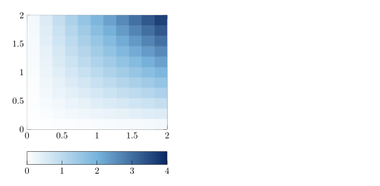
3D の視点
Scissor LaTeX は \addplot3 を真上から見た場合にのみ描きます。デフォルトの 3D の視点を含め、それ以外の view では軸が空のままになり、メッセージが表示されます。
3D の視点は描かれない
\begin{tikzpicture}
  \begin{axis}[width=6cm, height=5cm]
    \addplot3[surf, domain=-2:2, y domain=-2:2] {x^2 - y^2};
  \end{axis}
\end{tikzpicture}
「問題」タブ: 3D plots are drawn only when seen from above (view={0}{90}) for now
TeX のインストール環境との違い
\addplot3、カラーマップ、等高線の詳細は pgfplots のマニュアルにあります:ctan.org/pkg/pgfplots。
pgfplots の基本、対数軸、pgfplots もご覧ください。
よくある質問
LaTeX でヒートマップを作るにはどうすればよいですか?
view={0}{90} を指定した軸で \addplot3[surf, shader=interp] {f(x,y)};(表のデータなら matrix plot*)を使い、colorbar を追加します。
Scissor LaTeX で 3D の曲面グラフは描けますか?
まだ描けません。\addplot3 は真上から見た場合(view={0}{90})にのみ描かれ、ほかの視点では軸が空のままになり、「問題」タブにその旨が表示されます。
contour gnuplot で警告が出るのはなぜですか?
TeX のインストール環境では、gnuplot とシェルエスケープが必要だからです。Scissor LaTeX は等高線を描きますが、コードがほかの環境ではコンパイルできない可能性があると警告します。contour filled はどこでもコンパイルできます。
このページの例はすべて、サイトのビルド時に Scissor LaTeX で組版されています。 最終更新:2026-11-07