


等高线图、热力图和颜色映射
在带 view={0}{90} 的坐标轴中使用 \addplot3:热力图用 surf 或 matrix plot,填充等高线用 contour filled,再加上 colorbar 和一个 colormap 显示色标。
函数的热力图
\addplot3 绘制 x 和 y 的函数。从正上方看(view={0}{90}),surf 图就成了热力图:每个单元格按其数值通过颜色映射着色。shader=interp 让颜色平滑过渡;shader=flat 让每个单元格只有一种颜色。
带色标的平滑热力图
\begin{tikzpicture}
  \begin{axis}[view={0}{90}, colorbar, colormap/viridis,
               xlabel=$x$, ylabel=$y$, enlargelimits=false]
    \addplot3[surf, shader=interp, domain=-2:2, y domain=-2:2, samples=30]
      {exp(-x^2 - y^2) * (1 + x)};
  \end{axis}
\end{tikzpicture}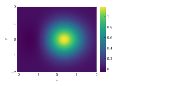
domain 设置 x 的范围,y domain 设置 y 的范围,samples 设置网格大小(默认 25;y 方向用不同数量时用 samples y)。
填充等高线图
contour filled 把数值划分为若干色带。number= 设置等高线的层数;levels={...} 可以自己列出各层。
双峰函数的填充等高线图
\begin{tikzpicture}
  \begin{axis}[view={0}{90}, colorbar, colormap/hot, enlargelimits=false]
    \addplot3[contour filled={number=8}, domain=-3:3, y domain=-3:3, samples=40]
      {exp(-(x-1)^2 - y^2) + 0.7*exp(-(x+1.2)^2 - (y-1)^2)};
  \end{axis}
\end{tikzpicture}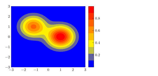
来自表格的热力图:matrix plot
对于网格上的测量数据,matrix plot* 为表格的每一行绘制一个单元格。mesh/cols 说明网格有多少列,point meta=explicit 配合 meta= 指定数值所在的列。
3 × 3 的数值网格
\begin{tikzpicture}
  \begin{axis}[colorbar, colormap/bluered, enlargelimits=false,
               xtick=data, ytick=data, width=6.5cm, height=6cm]
    \addplot[matrix plot*, mesh/cols=3, point meta=explicit]
      table[meta=v] {
        x y v
        0 0 1
        1 0 4
        2 0 2
        0 1 3
        1 1 9
        2 1 5
        0 2 2
        1 2 6
        2 2 44
      };
  \end{axis}
\end{tikzpicture}
等高线
不带填充的等高线需要替你计算等高线层级。在 pgfplots 中这对应 contour gnuplot 或 contour lua,在 TeX 发行版中它们需要额外的程序或 LuaLaTeX。Scissor LaTeX 会自己计算并绘制这些线,并在“问题”标签页中提醒你,这段代码可能无法在其他地方编译。
用 contour gnuplot 绘制的等高线
\begin{tikzpicture}
  \begin{axis}[view={0}{90}, xlabel=$x$, ylabel=$y$]
    \addplot3[contour gnuplot={levels={0.2, 0.5, 0.8}},
              domain=-2:2, y domain=-2:2, samples=30]
      {exp(-x^2 - y^2)};
  \end{axis}
\end{tikzpicture}
“问题”标签页: contour gnuplot needs gnuplot and shell escape in LaTeX; contour filled or contour prepared compile everywhere
如果文件要在任何地方都能编译,请使用 contour filled,或使用带预先计算的等高线数据的 contour prepared。
颜色映射和色标
| 选项 | 作用 | 在 Scissor LaTeX 中 |
|---|---|---|
colormap/viridis、/hot、/cool、/jet、/blackwhite、/bluered | 内置颜色映射 | 支持 |
colormap name=viridis | 按名称选择映射 | 支持 |
colormap={name}{rgb255=(..) rgb255=(..)} | 自定义映射 | 支持 |
colorbar、colorbar horizontal | 图表旁边或下方的色标 | 支持 |
colorbar style={..} | 色标的刻度和标签 | 支持 |
point meta min、point meta max | 固定颜色范围 | 支持 |
shader=flat、shader=interp、shader=faceted | 单元格的着色方式 | 支持 |
自定义颜色映射和水平色标
\begin{tikzpicture}
  \begin{axis}[view={0}{90}, enlargelimits=false,
               colormap={sea}{rgb255=(255,255,255) rgb255=(120,180,220) rgb255=(10,40,100)},
               colorbar horizontal, width=7cm, height=6cm]
    \addplot3[surf, shader=flat, domain=0:2, y domain=0:2, samples=12] {x*y};
  \end{axis}
\end{tikzpicture}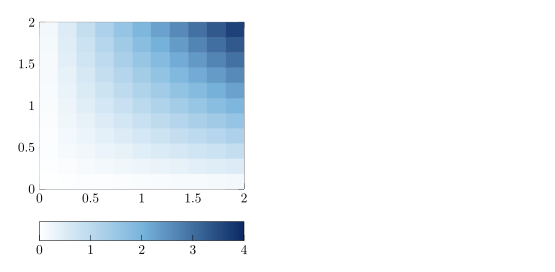
三维视角
Scissor LaTeX 只按从正上方俯视的视角绘制 \addplot3。其他任何 view,包括默认的三维视角,都会让坐标轴保持空白并给出提示。
三维视角不会被绘制
\begin{tikzpicture}
  \begin{axis}[width=6cm, height=5cm]
    \addplot3[surf, domain=-2:2, y domain=-2:2] {x^2 - y^2};
  \end{axis}
\end{tikzpicture}
“问题”标签页: 3D plots are drawn only when seen from above (view={0}{90}) for now
与 TeX 发行版的不同之处
pgfplots 手册详细介绍了 \addplot3、颜色映射和等高线:ctan.org/pkg/pgfplots。
另请参阅 pgfplots 基础、对数坐标轴和 pgfplots。
常见问题
如何在 LaTeX 中绘制热力图?
在带 view={0}{90} 的坐标轴中使用 \addplot3[surf, shader=interp] {f(x,y)};(表格数据则用 matrix plot*),并加上 colorbar。
Scissor LaTeX 能绘制三维曲面图吗?
暂时不能。\addplot3 只在从上方俯视(view={0}{90})时绘制;其他视角会让坐标轴保持空白,“问题”标签页会说明这一点。
为什么 contour gnuplot 会显示警告?
在 TeX 发行版中,它需要 gnuplot 和 shell escape。Scissor LaTeX 仍会绘制等高线,但会警告这段代码可能无法在其他地方编译。contour filled 在任何地方都能编译。
本页的每个示例都在构建网站时由 Scissor LaTeX 排版。 最后更新:2026-11-07