


pgfplots の散布図
pgfplots の axis の中の \addplot に only marks を追加すると、点が線なしで描かれます。形は mark= で選び、点は座標か表から読み込みます。
線のない点
散布図は、マーカーだけで描いた系列です。\addplot に only marks を追加し、+ を付けるとサイクルリストの色とマーカーが保たれます。
2 つのグループの点
\begin{tikzpicture}
  \begin{axis}[xlabel={Height (m)}, ylabel={Mass (kg)}, legend pos=north west]
    \addplot+[only marks] coordinates {
      (1.62,55) (1.68,61) (1.71,66) (1.75,69) (1.80,74) (1.84,79)};
    \addplot+[only marks] coordinates {
      (1.58,49) (1.64,57) (1.69,58) (1.73,64) (1.77,68)};
    \legend{Group A, Group B}
  \end{axis}
\end{tikzpicture}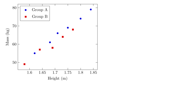
マーカーの形、大きさ、色
mark= で形を、mark size= で半径(デフォルトは 2pt)を指定します。塗りつぶした形は末尾が * です。mark options はマーカーだけのスタイルを指定し、たとえば白で塗った中抜きのマーカーにできます。
系列ごとに異なるマーカー
\begin{tikzpicture}
  \begin{axis}[enlargelimits=0.15, legend pos=outer north east]
    \addplot[only marks, mark=o, blue] coordinates {(1,2) (2,3) (3,2.5)};
    \addplot[only marks, mark=square*, red, mark size=3pt] coordinates {(1,1) (2,1.8) (3,1.2)};
    \addplot[only marks, mark=triangle*, teal, mark options={fill=white}] coordinates {(1,3) (2,4) (3,3.8)};
    \addplot[only marks, mark=x, black, mark size=4pt] coordinates {(1.5,0.5) (2.5,0.8)};
    \legend{circle, square, triangle, cross}
  \end{axis}
\end{tikzpicture}使える形は折れ線グラフのページに一覧があります。
表から読む点
点が多いときは、表として書きます。1 行目で列に名前を付け、x= と y= でプロットする列を選びます。表はここでのようにその場に書くことも、ファイルに置くこともできます(CSV ファイルのデータをご覧ください)。
その場に書いた表から読む点
\begin{tikzpicture}
  \begin{axis}[xlabel={Hours studied}, ylabel={Points}]
    \addplot[only marks, mark=*, blue!70!black] table[x=hours, y=points] {
      hours points
      2     21
      3     26
      4     30
      5     29
      6     37
      7     40
      8     44
    };
    \addplot[red, domain=2:8] {13.5 + 3.8*x};
  \end{axis}
\end{tikzpicture}
赤い線は点の上に重ねて描いた数式で、近似した傾向を簡単に示す方法です。
値に応じて点を色分けする
scatter を使うと、各点が値に応じてカラーマップから色付けされます。point meta=y は y の値を使い、scatter src=explicit と meta= を組み合わせると 3 つ目の列を読みます。colorbar を追加すると目盛りが表示されます。
3 つ目の列で色分けした点
\begin{tikzpicture}
  \begin{axis}[colorbar, colormap/viridis, xlabel=$x$, ylabel=$y$]
    \addplot[scatter, only marks, mark size=3pt, scatter src=explicit]
      table[x=x, y=y, meta=t] {
      x   y   t
      0.5 1.0 10
      1.0 2.2 15
      1.6 1.4 21
      2.1 3.0 28
      2.8 2.1 33
      3.3 3.6 44
    };
  \end{axis}
\end{tikzpicture}
点のクラス分け
pgfplots の scatter/classes は、列にあるクラス名ごとに独自のマーカーを割り当てます。Scissor LaTeX はまだこれに対応していません。オプションはメッセージ付きで無視され、すべての点が同じマーカーになります。
scatter/classes:すべての点が同じマーカー
\begin{tikzpicture}
  \begin{axis}[width=6cm, height=5cm]
    \addplot[scatter, only marks, scatter src=explicit symbolic,
             scatter/classes={a={mark=square*, blue}, b={mark=*, red}}]
      table[meta=group] {
      x y group
      1 1 a
      2 2 b
      3 1.5 a
    };
  \end{axis}
\end{tikzpicture}
「問題」タブ: pgfplots option 'scatter/classes' is not supported yet
TeX のインストール環境との違い
マーカーと散布図のオプションの詳細は pgfplots のマニュアルにあります:ctan.org/pkg/pgfplots。
よくある質問
線のない散布図を作るにはどうすればよいですか?
\addplot のオプションに only marks を追加します。たとえば \addplot+[only marks] coordinates {...}; です。
点の大きさを変えるにはどうすればよいですか?
\addplot に mark size=3pt を指定します。値はマーカーの半径です。
CSV ファイルの点をプロットできますか?
はい。ファイルをプロジェクトにアップロードし、\addplot+[only marks] table[x=a, y=b, col sep=comma] {file.csv}; と書きます。
このページの例はすべて、サイトのビルド時に Scissor LaTeX で組版されています。 最終更新:2026-11-07